Koopman

Controle Baseado em Dados

Prof. Dr. Raphael Teixeira

Universidade Federal do Pará

Notação

Objeto	Símbolo
Estado	\(\mathbf{x} \in \mathbb{R}^n\)
Dinâmica discreta / contínua	\(\mathbf{x}_{k+1} = \mathbf{F}(\mathbf{x}_k)\) / \(\dot{\mathbf{x}} = \mathbf{f}(\mathbf{x})\)
Observável genérico (escalar)	\(g(\mathbf{x})\)
Vetor de observáveis escolhidos	\(\mathbf{g}(\mathbf{x}) = [\,g_1(\mathbf{x}),\ \ldots,\ g_p(\mathbf{x})\,]^T\)
Operador de Koopman (discreto / contínuo)	\(\mathcal{K}\) / \(\mathcal{L}\)
Matriz que o representa (discreto / contínuo)	\(\mathbf{K}\) / \(\mathbf{L}\)
Autofunção e autovalor	\(\varphi_j(\mathbf{x})\) e \(\nu_j\)

Aviso

No exemplo deste material, \(\lambda\) e \(\mu\) são parâmetros do sistema. Por isso, os autovalores de Koopman são denotados por \(\nu\).

O que é um observável

Um observável é qualquer função escalar do estado:

\[ g : \mathbb{R}^n \to \mathbb{R} \]

Exemplos, com \(\mathbf{x} = [x_1,\ x_2]^T\):

• \(g(\mathbf{x}) = x_1\) (uma medição direta de um estado)
• \(g(\mathbf{x}) = x_1^2\) (por exemplo, proporcional a uma energia)
• \(g(\mathbf{x}) = x_1 x_2\) (por exemplo, uma potência)

• \(g\): um observável genérico, usado nas definições
• \(\mathbf{g}(\mathbf{x})\): um vetor de observáveis escolhidos
• \(\varphi_j\): observáveis especiais (autofunções), definidos adiante

O operador de Koopman

Tempo discreto: avaliar o observável um passo à frente.

\[ (\mathcal{K}g)(\mathbf{x}) = g\big(\mathbf{F}(\mathbf{x})\big) \qquad\Longleftrightarrow\qquad g(\mathbf{x}_{k+1}) = (\mathcal{K}g)(\mathbf{x}_k) \]

Tempo contínuo: a taxa de variação do observável ao longo da trajetória (regra da cadeia).

\[ \frac{d}{dt}\,g\big(\mathbf{x}(t)\big) = \nabla g(\mathbf{x}) \cdot \mathbf{f}(\mathbf{x}) =: (\mathcal{L}g)(\mathbf{x}) \]

Nota

O operador age sobre funções, não sobre o estado.

Por que ele é linear

Para quaisquer observáveis \(g_1\), \(g_2\) e escalares \(\alpha\), \(\beta\):

\[ \mathcal{K}(\alpha g_1 + \beta g_2)(\mathbf{x}) = \alpha\, g_1(\mathbf{F}(\mathbf{x})) + \beta\, g_2(\mathbf{F}(\mathbf{x})) = \alpha\,(\mathcal{K}g_1)(\mathbf{x}) + \beta\,(\mathcal{K}g_2)(\mathbf{x}) \]

• Vale mesmo que \(\mathbf{F}\) seja não linear
• A não linearidade continua lá, dentro da composição \(g \circ \mathbf{F}\)
• O que é linear é a regra “avaliar a função um passo à frente”

Dimensão infinita e subespaços invariantes

• \(\mathcal{K}\) age sobre o espaço de todas as funções do estado
• Esse espaço tem dimensão infinita: o operador também

Estratégia prática: procurar um subespaço invariante de dimensão finita

• gerado por observáveis \(g_1, \ldots, g_p\)
• que contenha os estados \(x_1, \ldots, x_n\)
• e que o operador não faça “sair” dele

Se existir, a restrição do operador a esse subespaço é uma matriz \(p \times p\).

O sistema

Sistema não linear de 2ª ordem, em tempo contínuo:

\[ \dot{x}_1 = \mu\, x_1, \qquad \dot{x}_2 = \lambda\,\left(x_2 - x_1^2\right) \]

• \(\mu < 0\) e \(\lambda < 0\), com \(|\lambda| \gg |\mu|\)
• \(x_1\) é lento; \(x_2\) é rápido
• A única não linearidade é o termo \(x_1^2\)
• Valores típicos: \(\mu = -0{,}05\), \(\lambda = -1\)

A escolha dos observáveis

Incluir a não linearidade como um novo observável:

\[ \mathbf{g}(\mathbf{x}) = \begin{bmatrix} g_1(\mathbf{x}) \\ g_2(\mathbf{x}) \\ g_3(\mathbf{x}) \end{bmatrix} = \begin{bmatrix} x_1 \\ x_2 \\ x_1^2 \end{bmatrix} \]

• \(g_1\) e \(g_2\) garantem que os estados estão no subespaço
• \(g_3\) é a não linearidade tratada como nova variável

A pergunta decisiva:

A derivada de cada \(g_i\) é uma combinação linear de \(g_1\), \(g_2\) e \(g_3\)?

O conjunto fecha

Aplicando \(\mathcal{L}g = \nabla g \cdot \mathbf{f}\) a cada observável:

\[ \mathcal{L}g_1 = \mu\, x_1 = \mu\, g_1 \]

\[ \mathcal{L}g_2 = \lambda\, x_2 - \lambda\, x_1^2 = \lambda\, g_2 - \lambda\, g_3 \]

\[ \mathcal{L}g_3 = 2x_1 \cdot \mu x_1 = 2\mu\, x_1^2 = 2\mu\, g_3 \]

Todas as derivadas ficaram dentro de \(\{g_1,\ g_2,\ g_3\}\): o subespaço é invariante.

O sistema levantado é linear e exato

\[ \frac{d}{dt} \underbrace{\begin{bmatrix} x_1 \\ x_2 \\ x_1^2 \end{bmatrix}}_{\mathbf{g}} = \underbrace{\begin{bmatrix} \mu & 0 & 0 \\ 0 & \lambda & -\lambda \\ 0 & 0 & 2\mu \end{bmatrix}}_{\mathbf{L}} \begin{bmatrix} x_1 \\ x_2 \\ x_1^2 \end{bmatrix} \]

• Nenhuma aproximação: é o sistema original, escrito em outras coordenadas
• \(\mathbf{L}\) representa \(\mathcal{L}\) restrito ao subespaço gerado por \(\{x_1,\ x_2,\ x_1^2\}\)
• Em tempo discreto, com período \(T_s\):

\[ \mathbf{g}(\mathbf{x}_{k+1}) = \mathbf{K}\,\mathbf{g}(\mathbf{x}_k), \qquad \mathbf{K} = e^{\mathbf{L}T_s} \]

Autovalores

\(\mathbf{L}\) é triangular superior: os autovalores estão na diagonal.

\[ \nu_1 = \mu, \qquad \nu_2 = \lambda, \qquad \nu_3 = 2\mu \]

• Um sistema de ordem 2 ganhou um terceiro modo
• \(2\mu\) não é um novo grau de liberdade físico
• É a taxa com que o observável \(x_1^2\) evolui: \(\left(x_1(0)\, e^{\mu t}\right)^2 = x_1(0)^2\, e^{2\mu t}\)

Nota

Produtos de observáveis geram combinações dos autovalores originais.

Autofunções de Koopman

Uma autofunção é um observável que evolui como um modo linear puro:

\[ \mathcal{L}\varphi = \nu\,\varphi \quad \Longrightarrow \quad \varphi\big(\mathbf{x}(t)\big) = \varphi\big(\mathbf{x}(0)\big)\, e^{\nu t} \]

No subespaço, \(\varphi(\mathbf{x}) = \mathbf{w}^T\mathbf{g}(\mathbf{x})\), em que \(\mathbf{w}\) é autovetor à esquerda de \(\mathbf{L}\):

\[ \mathbf{w}^T\mathbf{L} = \nu\,\mathbf{w}^T \]

Para \(\nu = \mu\) e \(\nu = 2\mu\), sai direto:

\[ \varphi_1(\mathbf{x}) = x_1, \qquad \varphi_3(\mathbf{x}) = x_1^2 \]

A autofunção de \(\nu = \lambda\)

Tentativa: \(\mathbf{w} = [\,0,\ 1,\ a\,]^T\)

\[ \mathbf{w}^T\mathbf{L} = \left[\,0,\ \ \lambda,\ \ -\lambda + 2\mu a\,\right] = \lambda\,\left[\,0,\ \ 1,\ \ a\,\right] \]

\[ -\lambda + 2\mu a = \lambda a \quad \Longrightarrow \quad a = -\frac{\lambda}{\lambda - 2\mu} \]

Definindo \(b = \dfrac{\lambda}{\lambda - 2\mu}\):

\[ \boxed{\ \varphi_2(\mathbf{x}) = x_2 - b\,x_1^2\ } \]

Verificação direta

\[ \mathcal{L}\varphi_2 = \dot{x}_2 - 2b\,x_1\dot{x}_1 = \lambda x_2 - \lambda x_1^2 - 2b\mu\, x_1^2 \]

\[ = \lambda x_2 - (\lambda + 2b\mu)\,x_1^2 \]

Com \(b(\lambda - 2\mu) = \lambda\), temos \(\lambda + 2b\mu = \lambda b\):

\[ \mathcal{L}\varphi_2 = \lambda\left(x_2 - b\,x_1^2\right) = \lambda\,\varphi_2 \quad \checkmark \]

Solução exata por álgebra linear

As autofunções evoluem de forma desacoplada:

\[ \varphi_1(t) = \varphi_1(0)\,e^{\mu t}, \qquad \varphi_2(t) = \varphi_2(0)\,e^{\lambda t} \]

Voltando às variáveis originais:

\[ x_1(t) = x_1(0)\,e^{\mu t} \]

\[ x_2(t) = b\,x_1(t)^2 + \left(x_2(0) - b\,x_1(0)^2\right)e^{\lambda t} \]

A solução do sistema não linear saiu sem integrar nenhuma EDO não linear.

Interpretação geométrica

O conjunto de nível \(\varphi_2 = 0\) é a parábola

\[ x_2 = b\,x_1^2 \]

• Como \(\lambda\) é rápido, \(\varphi_2 \to 0\) rapidamente: a trajetória cai na parábola
• Depois, desliza sobre ela com a dinâmica lenta de \(x_1\)
• Essa parábola é a variedade lenta do sistema
• Com \(|\lambda| \gg |\mu|\): \(b \approx 1\), logo \(x_2 \approx x_1^2\)

Dica

Autofunções são as coordenadas certas: em \((\varphi_1, \varphi_2)\), o sistema não linear vira dois modos lineares desacoplados.

Uma ressalva: ressonância

Se \(\lambda = 2\mu\):

• \(b = \dfrac{\lambda}{\lambda - 2\mu}\) não existe
• \(\mathbf{L}\) tem autovalor repetido e não é diagonalizável
• Aparece um termo secular do tipo \(t\,e^{\lambda t}\)

É o análogo, no espaço levantado, do caso de autovalores repetidos em sistemas lineares.

O que o exemplo ensina

1. Um observável é uma função do estado; o operador de Koopman age sobre observáveis
2. O operador é linear, mesmo para dinâmica não linear, mas de dimensão infinita
3. O modelo é exato quando se encontra um subespaço invariante finito que contém os estados
4. O modelo levantado tem mais modos que o sistema original
5. As autofunções são mudanças de coordenadas que linearizam o sistema
6. Estruturas triangulares (estado lento forçando estado rápido por termos polinomiais) sempre fecham

Quando o conjunto não fecha, é preciso aproximar dentro de um conjunto finito de observáveis escolhidos.

Verificação numérica (MATLAB)

mu = -0.05;  lambda = -1;
b  = lambda/(lambda - 2*mu);
L  = [mu 0 0; 0 lambda -lambda; 0 0 2*mu];

% Sistema nao linear (referencia)
f  = @(t,x) [mu*x(1); lambda*(x(2) - x(1)^2)];
x0 = [1.5; -1];  tf = 60;
[t, x] = ode45(f, [0 tf], x0, odeset('RelTol',1e-10,'AbsTol',1e-12));

% Sistema levantado linear: g(t) = expm(L t) g(0)
g0 = [x0(1); x0(2); x0(1)^2];
g  = zeros(3, numel(t));
for k = 1:numel(t)
    g(:,k) = expm(L*t(k))*g0;
end

% Comparacao no plano de fase
x1g = linspace(-2, 2, 200);
plot(x(:,1), x(:,2), 'k', 'LineWidth', 2); hold on;
plot(g(1,:), g(2,:), 'r--', 'LineWidth', 1.5);
plot(x1g, b*x1g.^2, 'b:', 'LineWidth', 1.5);
grid on; xlabel('x_1'); ylabel('x_2');
legend('Nao linear (ode45)', 'Koopman (linear)', 'Variedade lenta');
fprintf('Erro maximo: %.2e\n', max(abs(x.' - g(1:2,:)), [], 'all'));

Referências

S. L. Brunton, B. W. Brunton, J. L. Proctor, J. N. Kutz. Koopman invariant subspaces and finite linear representations of nonlinear dynamical systems for control. PLoS ONE, 11(2): e0150171, 2016.

S. L. Brunton, J. N. Kutz. Data-Driven Science and Engineering, capítulo sobre teoria de Koopman.

O que é o Operador de Koopman?

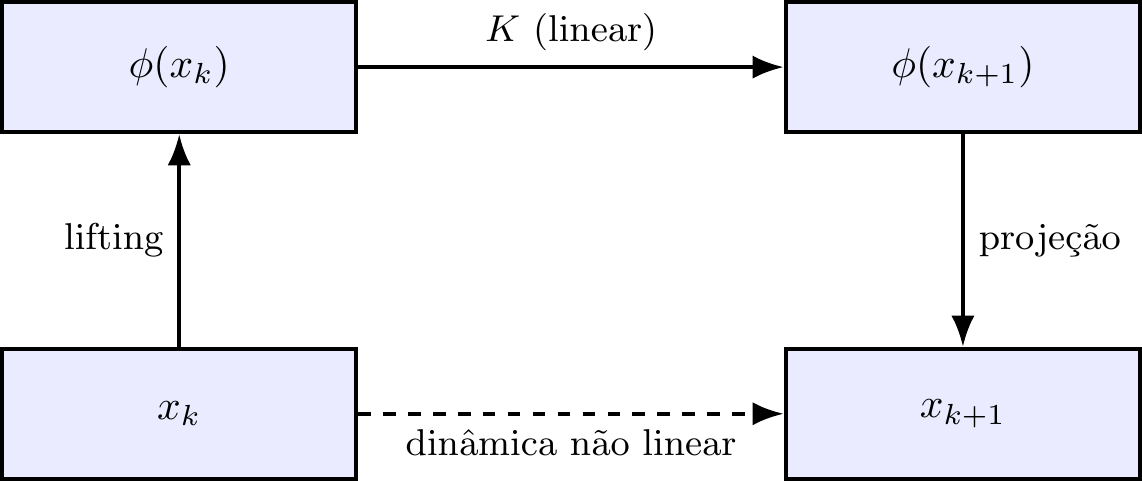
Um sistema não linear \(x_{k+1}=f(x_k)\) pode ser representado exatamente por um operador linear \(\mathcal{K}\), agindo sobre observáveis \(\phi(x)\) — ao custo de dimensão infinita (Koopman, 1931).

Motivação

• Controle linear (LQR, MPC linear) é maduro e barato de resolver;
• Controle não linear exige ferramentas mais caras;
• Ideia de Koopman: em vez de linearizar localmente (jacobiano), buscar coordenadas \(\phi(x)\) em que a dinâmica seja linear globalmente.

Definição do Operador

\(\mathcal{K}\) age sobre observáveis \(\phi:\mathcal{X}\to\mathbb{R}\) por \[(\mathcal{K}\phi)(x) = \phi(f(x))\] “Compor com \(f\)” é linear em \(\phi\), mesmo com \(f\) não linear.

O preço: \(\mathcal{K}\) atua num espaço de funções, de dimensão infinita, não sobre \(\mathcal{X}\) diretamente.

Autofunções e Modos de Koopman

Se \(\mathcal{K}\varphi=\lambda\varphi\), então \(\varphi(x_{k+1})=\lambda\,\varphi(x_k)\) ao longo de qualquer trajetória — a autofunção evolui linearmente.

Expandindo \(x=\sum_i \varphi_i(x)\,v_i\) (os \(v_i\) são os modos de Koopman):

\[ x_k = \sum_i \lambda_i^k\, \varphi_i(x_0)\, v_i \]

Solução explícita, análoga a \(\dot x=Ax\), mas para o sistema não linear (Mezić, 2005).

Da Teoria à Prática: DMD e EDMD

DMD (Schmid, 2010): usa \(\phi(x)=x\), ajusta \(A\) tal que \(x_{k+1}\approx Ax_k\). Só funciona se a dinâmica já for quase linear.

EDMD (Williams; Kevrekidis; Rowley, 2015): enriquece com uma biblioteca \(\phi_1,\dots,\phi_n\) (monômios, RBFs, …) e ajusta \(K\) por mínimos quadrados:

\[ K = \arg\min_{K} \sum_{k} \| \phi(x_{k+1}) - K\, \phi(x_k) \|_2^2 \]

Da Identificação ao Controle

Com o preditor linear \(z_{k+1}=Kz_k+Bu_k\) (\(z=\phi(x)\)), técnicas lineares se aplicam a uma planta não linear:

• LQR e MPC linear com restrições, em vez de MPC não linear (Korda; Mezić, 2018);
• Variante com kernels, para bibliotecas de dimensão muito alta (Williams; Rowley; Kevrekidis, 2015).

Importante

A escolha da biblioteca de observáveis determina a qualidade do controlador — não há receita universal (Brunton et al., 2022).

Referências

BRUNTON, Steven L. et al. Modern Koopman Theory for Dynamical Systems. SIAM Review, v. 64, n. 2, p. 229–340, 2022.

KOOPMAN, Bernard O. Hamiltonian Systems and Transformation in Hilbert Space. Proceedings of the National Academy of Sciences, v. 17, n. 5, p. 315–318, 1931.

KORDA, Milan; MEZIĆ, Igor. Linear Predictors for Nonlinear Dynamical Systems: Koopman Operator Meets Model Predictive Control. Automatica, v. 93, p. 149–160, 2018.

MEZIĆ, Igor. Spectral Properties of Dynamical Systems, Model Reduction and Decompositions. Nonlinear Dynamics, v. 41, p. 309–325, 2005.

SCHMID, Peter J. Dynamic Mode Decomposition of Numerical and Experimental Data. Journal of Fluid Mechanics, v. 656, p. 5–28, 2010.

WILLIAMS, Matthew O.; KEVREKIDIS, Ioannis G.; ROWLEY, Clarence W. A Data-Driven Approximation of the Koopman Operator: Extending Dynamic Mode Decomposition. Journal of Nonlinear Science, v. 25, p. 1307–1346, 2015.

WILLIAMS, Matthew O.; ROWLEY, Clarence W.; KEVREKIDIS, Ioannis G. A Kernel-Based Method for Data-Driven Koopman Spectral Analysis. Journal of Computational Dynamics, v. 2, n. 2, p. 247–265, 2015.

Encerramento

Prof. Dr. Raphael Teixeira

Universidade Federal do Pará

raphaelbt@ufpa.br