import pandas as pd
import numpy as np
import matplotlib.pyplot as plt
import seaborn as sns
import plotly.express as px

#Montar o drive:
from google.colab import drive
drive.mount('/content/drive')

Mounted at /content/drive

#arquivo = "/content/drive/MyDrive/Mestrado/Mestrado_Otacílio_Raphael/DataSetDGA/DataSet_DGA_(Rev1)T1.xlsx"
arquivo = "/content/drive/MyDrive/Mestrado/Mestrado_Otacílio_Raphael/DataSetDGA/DataSetDGA(Rev1)T1_S.Outiliers.xlsx"

DataSet = pd.read_excel(arquivo)                                                                          # Sintaxe para nomear DataSet.
DataSet.head()

	Unnamed: 0	H2	CH4	C2H4	C2H6	C2H2	NTE	NF	Rótulo
0	0	21.00	63.0	4.0	87.0	1.0	0	0	NO
1	1	0.01	61.0	6.0	81.0	1.0	0	0	NO
2	2	0.01	58.0	5.0	77.0	1.0	0	0	NO
3	3	0.01	56.0	6.0	73.0	1.0	0	0	NO
4	4	0.01	58.0	5.0	75.0	1.0	0	0	NO

gases = ['H2', 'CH4', 'C2H4', 'C2H6', 'C2H2']
X = DataSet[gases].values
m, n = X.shape

xmax = np.max(X,axis = 0)
xmin = np.min(X,axis = 0)
print('Valores máximos:', xmax)
print('Valores mínimos:', xmin)

Valores máximos: [22566. 64064. 95650. 72128. 57000.]
Valores mínimos: [0.01 0.01 0.01 0.01 0.01]

Xl = np.log(X)
#Xn = np.log(X)

# Normalizar DataSet:
from sklearn.preprocessing import StandardScaler
Xn = StandardScaler().fit_transform(Xl)
print('Média antes:',np.mean(X))
print('Média depois:',np.mean(Xn))
print('Variância antes:',np.std(X))
print('Variância depois:',np.std(Xn))
np.isnan(Xn)

Média antes: 138.30720459081837
Média depois: -6.52394527843605e-17
Variância antes: 1617.3875441693656
Variância depois: 0.9999999999999999

array([[False, False, False, False, False],
       [False, False, False, False, False],
       [False, False, False, False, False],
       ...,
       [False, False, False, False, False],
       [False, False, False, False, False],
       [False, False, False, False, False]])

y = DataSet['NTE'].values

from sklearn.model_selection import train_test_split

X_train, X_test, y_train, y_test = train_test_split(Xn, y, test_size=0.33, random_state=101)

from sklearn.neighbors import KNeighborsClassifier

A = np.array([])
vizinhos = np.arange(1, 50, 2)
for n in vizinhos:
  knn = KNeighborsClassifier(n_neighbors=n,  weights='uniform', algorithm='auto', leaf_size=30, p=2, metric='minkowski', metric_params=None, n_jobs=None)
  knn.fit(X_train, y_train)
  pred = knn.predict(X_test)
  A = np.append(A, np.sum(pred==y_test)/len(pred))

plt.figure(figsize = (7, 4))
plt.plot(vizinhos, A)
plt.plot(vizinhos, A, 'rx')
plt.title("K-Vizinho Ideal",fontsize=10)
plt.xlabel('K-Vizinhos',fontsize=10)
plt.ylabel('Desempenho',fontsize=10)
plt.grid()
plt.ylim((0.9, 1))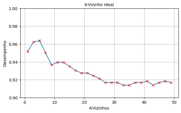

knn = KNeighborsClassifier(n_neighbors=5,  weights='uniform', algorithm='auto', leaf_size=30, p=2, metric='minkowski', metric_params=None, n_jobs=None)
knn.fit(X_train, y_train)
pred = knn.predict(X_test)

pred.shape

(662,)

from sklearn.metrics import classification_report, confusion_matrix

print(classification_report(y_test, pred))
print(confusion_matrix(y_test, pred))

              precision    recall  f1-score   support

           0       0.96      0.99      0.97       442
           1       0.94      0.91      0.93       129
           2       0.95      0.87      0.91        91

    accuracy                           0.96       662
   macro avg       0.95      0.92      0.94       662
weighted avg       0.96      0.96      0.96       662

[[436   4   2]
 [  9 118   2]
 [  9   3  79]]

np.sum(pred==y_test)/len(pred)

0.9637462235649547

from sklearn.metrics import cohen_kappa_score

E1 = y_test

E1.shape

(662,)

E2 = pred

E2.shape

(662,)

K_Knn = cohen_kappa_score(E1,E2, weights = 'linear')

K_Knn

0.9255079006772009

E3.shape

(662,)

K_Knn2 = cohen_kappa_score(E3,E4, weights = 'linear')

K_Knn2

0.9255079006772009