Controle Digital
5 figura(s) nesta categoria. Fonte em figuras/controle-digital/.
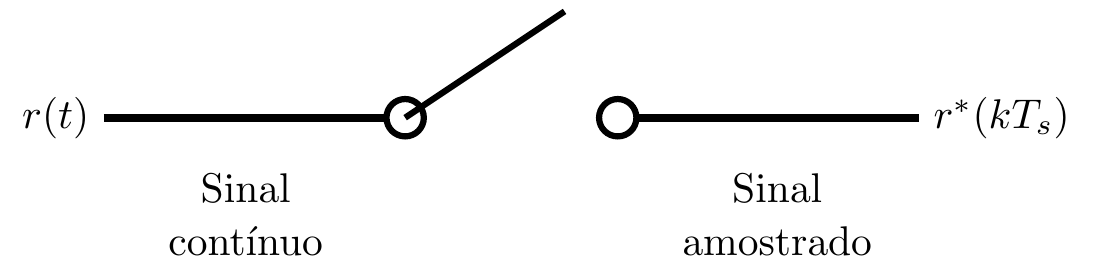
Amostrador ideal
Chave amostradora que converte um sinal contínuo r(t) num sinal amostrado r*(kTs).
Ver código TikZ
\begin{tikzpicture}[scale=1.5, every node/.style={font=\normalsize}]
  % Input signal line
  \draw[line width=2pt] (0,0) -- (1.6,0);
  \node[below=0.35cm] at (0.8,0) {Sinal};
  \node[below=0.8cm] at (0.8,0) {contínuo};
  \node[left] at (0,0) {$r(t)$};

  % Left terminal (contact point)
  \draw[line width=1.5pt, fill=white] (1.7,0) circle (3pt);

  % Switch arm (chave) - diagonal open
  \draw[line width=1.5pt] (1.7,0) -- (2.6,0.6);

  % Right terminal (contact point)
  \draw[line width=1.5pt, fill=white] (2.9,0) circle (3pt);

  % Output signal line
  \draw[line width=2pt] (3.0,0) -- (4.6,0);
  \node[below=0.35cm] at (3.8,0) {Sinal};
  \node[below=0.8cm] at (3.8,0) {amostrado};
  \node[right] at (4.6,0) {$r^*(kT_s)$};
\end{tikzpicture}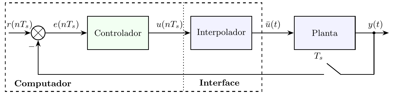
Malha de Controle com Sinal Amostrado
Diagrama de blocos de uma malha de controle digital destacando o amostrador entre o controlador discreto e a planta contínua.
Ver código TikZ
\begin{tikzpicture}[
    auto,
    node distance=1.5cm,
    block/.style={draw, fill=blue!5, rectangle, minimum height=1.2cm, minimum width=2.2cm, align=center, thick},
    block_ctrl/.style={draw, fill=green!5, rectangle, minimum height=1.2cm, minimum width=2.2cm, align=center, thick},
    sum/.style={draw, circle, minimum size=0.5cm, thick},
    arrow/.style={-Stealth, thick},
    dot/.style={fill, circle, minimum size=3pt, inner sep=0pt},
    every node/.style={font=\small}
]

    % --- Nós ---
    \node (input) {};
    \node [sum, right=0.8cm of input] (sum) {};
    \node [block_ctrl, right=of sum] (controller) {Controlador};
    \node [block, right=of controller] (interpolator) {Interpolador};
    \node [block, right=1.5cm of interpolator] (plant) {Planta};
    \node [right=1.2cm of plant] (output) {};

    % --- Caminho Direto ---
    \draw [arrow] (input) -- node {$r(nT_s)$} (sum);
    \draw (sum.north east) -- (sum.south west);
    \draw (sum.north west) -- (sum.south east);

    \draw [arrow] (sum) -- node {$e(nT_s)$} (controller);
    \draw [arrow] (controller) -- node {$u(nT_s)$} (interpolator);
    \draw [arrow] (interpolator) -- node {$\bar{u}(t)$} (plant);
    \draw [arrow] (plant) -- node [pos=0.6] (c_node) {$y(t)$} (output);

    % --- Realimentação ---
    \node [dot] at ($(plant.east)!0.5!(output)$) (branch) {};

    % Desce da ramificação
    \draw [thick] (branch) |- ++(0,-1.5) coordinate (corner);
    % Linha horizontal até a chave
    \draw [thick] (corner) -- ++(-1.2,0) coordinate (sampler_tip);

    % Chave (amostrador) com T_s (sem a seta curva)
    \draw [thick] (sampler_tip) -- ++(-0.5,0.4) node[above left] {$T_s$};

    % O fechamento:
    \draw [arrow] ($(sampler_tip)+(-0.6,0)$) -| (sum.south)
        node[pos=0.9, left] {\textbf{--}};

    % --- Containers (Medidas Originais) ---
    \draw [dashed, thick] ($(sum.north west)+(-1.0,0.9)$) rectangle ($(interpolator.south east)+(0.35,-1.5)$);
    \draw [dotted, thick] ($(controller.north east)+(1.25,0.49)$) -- ($(controller.south east)+(1.25,-1.5)$);

    % Rótulos
    \node [anchor=south west] at ($(sum.north west)+(-0.8,-2.3)$) {\textbf{Computador}};
    \node [anchor=north west] at ($(controller.south east)+(1.7,-0.95)$) {\textbf{Interface}};

\end{tikzpicture}
Malha de Controle Digital
Diagrama de blocos de malha fechada com controlador e planta discretos, no domínio Z.

Ver código TikZ
\begin{tikzpicture}[
    auto,
    % Distância padrão entre os nós para compactar
    node distance=1.6cm,
    % Estilo padrão para blocos (Planta)
    block/.style={draw, fill=blue!5, rectangle, minimum height=1.2cm, minimum width=2.2cm, align=center, thick},
    % Estilo específico para o Controlador (cor diferente)
    block_ctrl/.style={draw, fill=green!5, rectangle, minimum height=1.2cm, minimum width=2.2cm, align=center, thick},
    % Estilo para o ponto de soma (menor)
    sum/.style={draw, circle, minimum size=0.5cm, thick},
    % Estilo para as setas
    arrow/.style={-Stealth, thick},
    % Ponto de derivação
    dot/.style={fill, circle, minimum size=3pt, inner sep=0pt},
    % Define o tamanho da fonte padrão para os rótulos
    every node/.style={font=\small}
]

    % --- Nós ---
    \node (input) {};
    % Aproximei o ponto de soma da entrada
    \node [sum, right=0.8cm of input] (sum) {};

    % Controlador (usando o estilo block_ctrl)
    \node [block_ctrl, right=of sum] (controller) {Controlador \\ $C(z)$};

    % Planta
    \node [block, right=of controller] (plant) {Planta \\ $G(z)$};

    % Reduzi o tamanho da seta de saída para compactar
    \node [right=1.8cm of plant] (output) {};

    % --- Caminho Direto ---
    % Removido o nó que continha o sinal de "+" na entrada
    \draw [arrow] (input) -- node {$R(z)$} (sum);

    \draw [arrow] (sum) -- node {$E(z)$} (controller);

    \draw [arrow] (controller) -- node {$U(z)$} (plant);

    % Posição do rótulo de saída ajustada
    \draw [arrow] (plant) -- node (y_out) [pos=0.6] {$Y(z)$} (output);

    % --- Realimentação (Feedback) ---
    % Ponto de ramificação ajustado para a saída menor
    \node [dot, right=1.0cm of plant] (branch) {};

    % Caminho de volta mais próximo e com sinal '-' deslocado
    \draw [thick] (branch) |- ++(0,-1.3) -| node[pos=0.95, xshift=0.4cm] {\textbf{--}} (sum);

    % Detalhe interno do ponto de soma
    \draw (sum.north east) -- (sum.south west);
    \draw (sum.north west) -- (sum.south east);

\end{tikzpicture}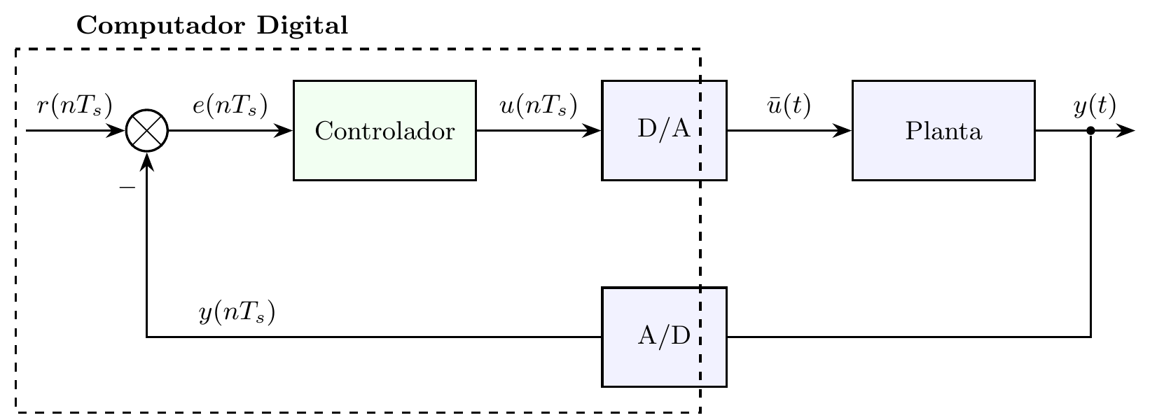
Malha de Controle Digital (Domínio do Tempo Discreto)
Diagrama de blocos de malha fechada digital com sinais no domínio do tempo discreto (amostras k).
Ver código TikZ
\begin{tikzpicture}[
    auto,
    node distance=1.5cm,
    block/.style={draw, fill=blue!5, rectangle, minimum height=1.2cm, minimum width=2.2cm, align=center, thick},
    block_ctrl/.style={draw, fill=green!5, rectangle, minimum height=1.2cm, minimum width=2.2cm, align=center, thick},
    sum/.style={draw, circle, minimum size=0.5cm, thick},
    arrow/.style={-Stealth, thick},
    dot/.style={fill, circle, minimum size=3pt, inner sep=0pt},
    every node/.style={font=\small}
]

    % --- Nós ---
    \node (input) {};
    \node [sum, right=1.2cm of input] (sum) {};
    \node [block_ctrl, right=of sum] (controller) {Controlador};

    % Conversor D/A
    \node [block, right=1.5cm of controller, minimum width=1.5cm] (da) {D/A};

    % Planta
    \node [block, right=1.5cm of da] (plant) {Planta};
    \node [right=1.2cm of plant] (output) {};

    % --- Caminho Direto ---
    \draw [arrow] (input) -- node {$r(nT_s)$} (sum);
    \draw (sum.north east) -- (sum.south west);
    \draw (sum.north west) -- (sum.south east);

    \draw [arrow] (sum) -- node {$e(nT_s)$} (controller);
    \draw [arrow] (controller) -- node {$u(nT_s)$} (da);
    \draw [arrow] (da) -- node {$\bar{u}(t)$} (plant);
    \draw [arrow] (plant) -- node [pos=0.6] (c_node) {$y(t)$} (output);

    % --- Realimentação com A/D Alinhado ---
    \node [dot] at ($(plant.east)!0.5!(output)$) (branch) {};

    % Posicionando o A/D exatamente abaixo do D/A
    \node [block, minimum width=1.5cm] at (da.center |- 0,-2.5) (ad) {A/D};

    % Caminho da realimentação
    \draw [thick] (branch) |- (ad);
    \draw [arrow] (ad) -| (sum.south)
        node [pos=0.4, above] {$y(nT_s)$}
        node [pos=0.9, left] {\textbf{--}};

    % --- Container do Computador Digital ---
    % Ajustado para englobar a referência interna e o caminho de volta
    \draw [dashed, thick] ($(sum.north west)+(-1.4,0.8)$) rectangle ($(controller.south east)+(2.7,-2.8)$);

    % Rótulo do Computador
    \node [anchor=south west] at ($(sum.north west)+(-0.8,0.8)$) {\textbf{Computador Digital}};

\end{tikzpicture}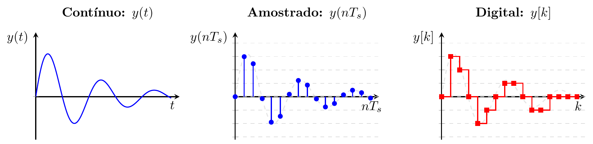
Sinais Contínuo, Amostrado e Digital
Três gráficos lado a lado comparando o mesmo sinal em suas representações contínua y(t), amostrada y(nTs) e digital/quantizada y[k].
Ver código TikZ
\begin{tikzpicture}
    % Configurações compartilhadas
    \pgfplotsset{
        my_axis_style/.style={
            width=5.5cm, height=4.5cm,
            axis lines=middle,
            xmin=0, xmax=8.5,
            ymin=-0.8, ymax=1.2,
            % Remove números e marcas dos eixos
            xtick=\empty,
            ytick={-0.75,-0.5,-0.25,0.25,0.5,0.75,1.0},
            yticklabels=\empty,
            extra y ticks={0},
            extra y tick labels=\empty,
            domain=0:8,
            samples=100,
            thick,
            % Rótulo do eixo Y à esquerda
            every axis y label/.style={at={(ticklabel* cs:0.95)}, anchor=east, xshift=-2pt},
            every axis x label/.style={at={(ticklabel* cs:0.95)}, anchor=north}
        }
    }

    % 1. Sinal Contínuo y(t)
    \begin{axis}[
        my_axis_style,
        title={\textbf{Contínuo: $y(t)$}},
        name=cont,
        ylabel={$y(t)$},
        xlabel={$t$},
        ytick=\empty % Sem grid no contínuo
    ]
        \addplot[blue, smooth] {exp(-0.3*x)*sin(deg(2*x))};
    \end{axis}

    % 2. Sinal Amostrado y(nTs)
    \begin{axis}[
        my_axis_style,
        title={\textbf{Amostrado: $y(nT_s)$}},
        name=amost,
        at={(cont.right of south east)},
        xshift=1.5cm,
        anchor=south west,
        ylabel={$y(nT_s)$},
        xlabel={$nT_s$},
        % Correção do Grid
        ymajorgrids=true,
        grid style={dashed, gray!30}
    ]
        \addplot[gray, dashed, opacity=0.2] {exp(-0.3*x)*sin(deg(2*x))};
        \addplot[blue, ycomb, samples=16, mark=*, mark size=1.5pt] {exp(-0.3*x)*sin(deg(2*x))};
    \end{axis}

    % 3. Sinal Digital yq[k]
    \begin{axis}[
        my_axis_style,
        title={\textbf{Digital: $y[k]$}},
        name=dig,
        at={(amost.right of south east)},
        xshift=1.5cm,
        anchor=south west,
        ylabel={$y[k]$},
        xlabel={$k$},
        % Correção do Grid
        ymajorgrids=true,
        grid style={dashed, gray!30}
    ]
        \addplot[gray, dashed, opacity=0.2] {exp(-0.3*x)*sin(deg(2*x))};
        \addplot[red, const plot, samples=16, mark=square*, mark size=1.5pt] {round(exp(-0.3*x)*sin(deg(2*x))*4)/4};
    \end{axis}

\end{tikzpicture}