Álgebra Linear
7 figura(s) nesta categoria. Fonte em figuras/algebra-linear/.
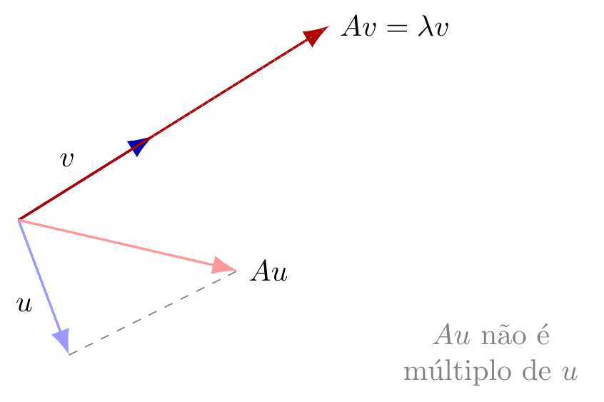
Autovetor: direção preservada sob transformação
Vetor v e sua imagem Av=λv na mesma direção (autovetor), contrastados com um vetor genérico u cuja imagem Au não é múltiplo de u.
Ver código TikZ
\begin{tikzpicture}[vec/.style={-{Latex[length=3mm]}, thick}, >=Latex]

  \coordinate (O) at (0,0);

  % --- Autovetor v e sua imagem Av = lambda v (mesma direcao) ---
  \coordinate (V) at (1.6,1.0);
  \coordinate (AV) at (3.68,2.3);

  \draw[vec, blue!70!black] (O) -- (V) node[midway, above left, black] {$v$};
  \draw[vec, red!70!black] (O) -- (AV) node[right, black] {$Av=\lambda v$};
  \draw[dotted, gray] (V) -- (AV);

  % --- Vetor generico u e sua imagem Au (direcao diferente) ---
  \coordinate (U) at (0.6,-1.6);
  \coordinate (AU) at (2.6,-0.6);

  \draw[vec, blue!40!white] (O) -- (U) node[midway, below left, black] {$u$};
  \draw[vec, red!40!white] (O) -- (AU) node[right, black] {$Au$};
  \draw[dashed, gray] (U) -- (AU);

  \node[gray, align=center] at (5.6,-1.6) {$Au$ não é\\múltiplo de $u$};

\end{tikzpicture}
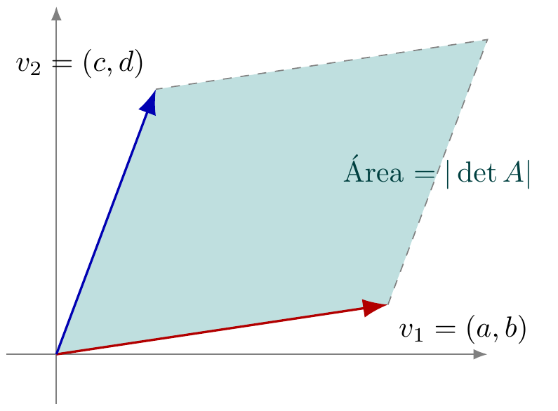
Determinante como área
Paralelogramo formado por dois vetores-coluna v1=(a,b) e v2=(c,d) a partir da origem, ilustrando que a área da figura é igual ao valor absoluto do determinante da matriz formada pelos vetores.
Ver código TikZ
\begin{tikzpicture}[vec/.style={-{Latex[length=3mm]}, thick}, >=Latex]
  \coordinate (O) at (0,0);
  \coordinate (A) at (4,0.6);
  \coordinate (B) at (1.2,3.2);
  \coordinate (C) at ($(A)+(B)$);

  \fill[teal!25] (O) -- (A) -- (C) -- (B) -- cycle;

  \draw[->, gray] (-0.6,0) -- (5.2,0);
  \draw[->, gray] (0,-0.6) -- (0,4.2);

  \draw[dashed, gray] (A) -- (C) -- (B);

  \draw[vec, red!70!black] (O) -- (A) node[below right, black] {$v_1=(a,b)$};
  \draw[vec, blue!70!black] (O) -- (B) node[above left, black] {$v_2=(c,d)$};

  \node[teal!50!black] at ($(A)!0.5!(C)$) {Área $=|\det A|$};
\end{tikzpicture}
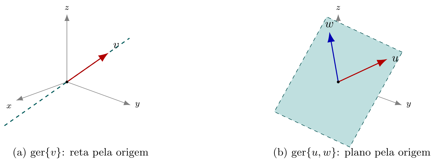
Espaço gerado por um e por dois vetores
Dois painéis com eixos pseudo-3D: (a) um vetor não nulo v e a reta que ele gera pela origem; (b) dois vetores LI u,w e o plano que eles geram pela origem.
Ver código TikZ
\begin{tikzpicture}[vec/.style={-{Latex[length=3mm]}, thick}, >=Latex]

% ---------- Painel (a): reta gerada por um vetor ----------
\begin{scope}
  \coordinate (O) at (0,0);
  \coordinate (Xax) at (200:1.6);
  \coordinate (Yax) at (-20:2.0);
  \coordinate (Zax) at (90:2.0);

  % eixos pseudo-3D
  \draw[gray, -{Latex[length=2mm]}] (O) -- (Xax) node[below left, black] {\scriptsize $x$};
  \draw[gray, -{Latex[length=2mm]}] (O) -- (Yax) node[right, black] {\scriptsize $y$};
  \draw[gray, -{Latex[length=2mm]}] (O) -- (Zax) node[above, black] {\scriptsize $z$};

  \coordinate (V) at (35:1.5);

  % reta gerada por v (estendida nos dois sentidos)
  \draw[teal!70!black, thick, dashed] ($-1.5*(V)$) -- ($1.5*(V)$);

  \draw[vec, red!70!black] (O) -- (V) node[above right, black] {$v$};
  \fill (O) circle (1.2pt);

  \node[align=center] at (0.4,-2.1) {\small (a) $\mathrm{ger}\{v\}$: reta pela origem};
\end{scope}

% ---------- Painel (b): plano gerado por dois vetores LI ----------
\begin{scope}[xshift=8cm]
  \coordinate (O) at (0,0);
  \coordinate (Xax) at (200:1.6);
  \coordinate (Yax) at (-20:2.0);
  \coordinate (Zax) at (90:2.0);

  \draw[gray, -{Latex[length=2mm]}] (O) -- (Xax) node[below left, black] {\scriptsize $x$};
  \draw[gray, -{Latex[length=2mm]}] (O) -- (Yax) node[right, black] {\scriptsize $y$};
  \draw[gray, -{Latex[length=2mm]}] (O) -- (Zax) node[above, black] {\scriptsize $z$};

  \coordinate (U) at (25:1.6);
  \coordinate (W) at (100:1.5);

  % plano gerado por u e w: paralelogramo com diagonais U-(-U) e W-(-W)
  \fill[teal!25] ($1.3*(U)$) -- ($1.3*(W)$) -- ($-1.3*(U)$) -- ($-1.3*(W)$) -- cycle;
  \draw[teal!60!black, dashed] ($1.3*(U)$) -- ($1.3*(W)$) -- ($-1.3*(U)$) -- ($-1.3*(W)$) -- cycle;

  \draw[vec, red!70!black] (O) -- (U) node[right, black] {$u$};
  \draw[vec, blue!70!black] (O) -- (W) node[above, black] {$w$};
  \fill (O) circle (1.2pt);

  \node[align=center] at (0.4,-2.1) {\small (b) $\mathrm{ger}\{u,w\}$: plano pela origem};
\end{scope}

\end{tikzpicture}
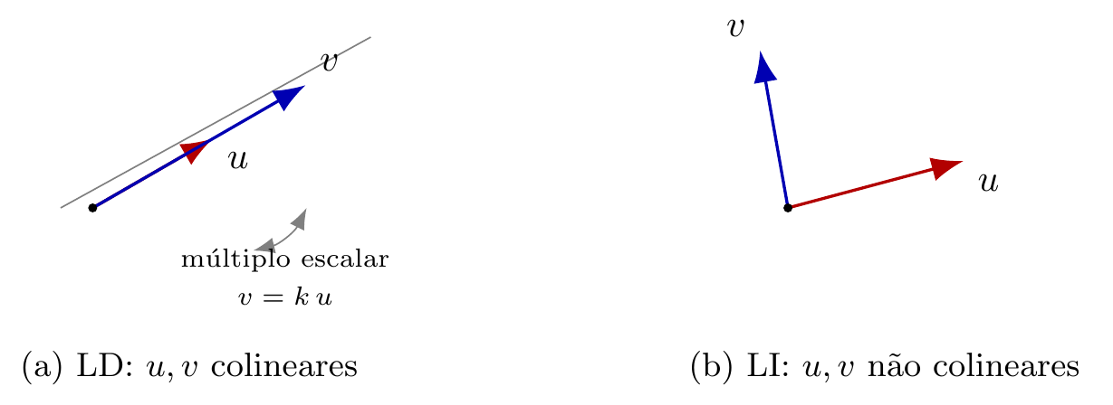
Dependência vs. independência linear
Dois painéis contrastando vetores linearmente dependentes (colineares, v = k·u) e linearmente independentes (não colineares) em R².
Ver código TikZ
\begin{tikzpicture}[vec/.style={-{Latex[length=3mm]}, thick}, >=Latex]

% ---------- Painel (a): vetores LD (colineares) ----------
\begin{scope}
  \coordinate (O) at (0,0);
  \draw[gray] (-0.3,0) -- (2.6,1.6);

  \coordinate (U) at (30:1.3);
  \coordinate (V) at (30:2.3);

  \draw[vec, red!70!black] (O) -- (U) node[below right, black] {$u$};
  \draw[vec, blue!70!black] (O) -- (V) node[above right, black] {$v$};
  \fill (O) circle (1.2pt);

  \draw[{Latex[length=2mm]}-{Latex[length=2mm]}, gray] (1.5,-0.4) to[bend right=25] node[below,black,align=center] {\scriptsize múltiplo escalar\\[-2pt]\scriptsize $v = k\,u$} (2.0,0.0);

  \node[align=center] at (0.9,-1.5) {\small (a) LD: $u,v$ colineares};
\end{scope}

% ---------- Painel (b): vetores LI (não colineares) ----------
\begin{scope}[xshift=6.5cm]
  \coordinate (O) at (0,0);

  \coordinate (A) at (15:1.7);
  \coordinate (B) at (100:1.5);

  \draw[vec, red!70!black] (O) -- (A) node[below right, black] {$u$};
  \draw[vec, blue!70!black] (O) -- (B) node[above left, black] {$v$};
  \fill (O) circle (1.2pt);

  \node[align=center] at (0.9,-1.5) {\small (b) LI: $u,v$ não colineares};
\end{scope}

\end{tikzpicture}
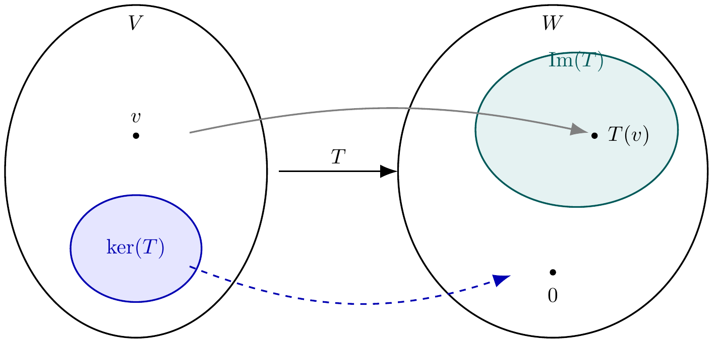
Núcleo e imagem de uma transformação linear
Diagrama esquemático de uma transformação linear T:V→W, mostrando o núcleo ker(T) dentro de V mapeado na origem de W, e a imagem Im(T) dentro de W.
Ver código TikZ
\begin{tikzpicture}[vec/.style={-{Latex[length=3mm]}, thick}, >=Latex]
  % Domain V
  \draw[thick] (0,0) ellipse (2.2 and 2.8);
  \node at (0,2.5) {$V$};

  % ker(T) blob inside V
  \draw[thick, blue!70!black, fill=blue!10] (0,-1.3) ellipse (1.1 and 0.9);
  \node[blue!70!black] at (0,-1.3) {$\ker(T)$};

  % generic vector v in V
  \fill (0,0.6) circle (1.5pt);
  \node[above] at (0,0.7) {$v$};

  % Codomain W
  \draw[thick] (7,0) ellipse (2.6 and 2.8);
  \node at (7,2.5) {$W$};

  % Im(T) blob inside W
  \draw[thick, teal!70!black, fill=teal!10] (7.4,0.7) ellipse (1.7 and 1.3);
  \node[teal!70!black] at (7.4,1.85) {$\mathrm{Im}(T)$};

  % origin point in W (image of ker)
  \fill (7,-1.7) circle (1.5pt);
  \node[below] at (7,-1.85) {$0$};

  % image of v
  \fill (7.7,0.6) circle (1.5pt);
  \node[right] at (7.8,0.6) {$T(v)$};

  % main arrow T
  \draw[vec] (2.4,0) -- (4.4,0) node[midway, above] {$T$};

  % ker(T) -> 0 arrow
  \draw[vec, blue!70!black, dashed] (0.9,-1.6) to[bend right=20] (6.3,-1.75);

  % v -> T(v) arrow
  \draw[vec, gray] (0.9,0.65) to[bend left=12] (7.6,0.65);
\end{tikzpicture}
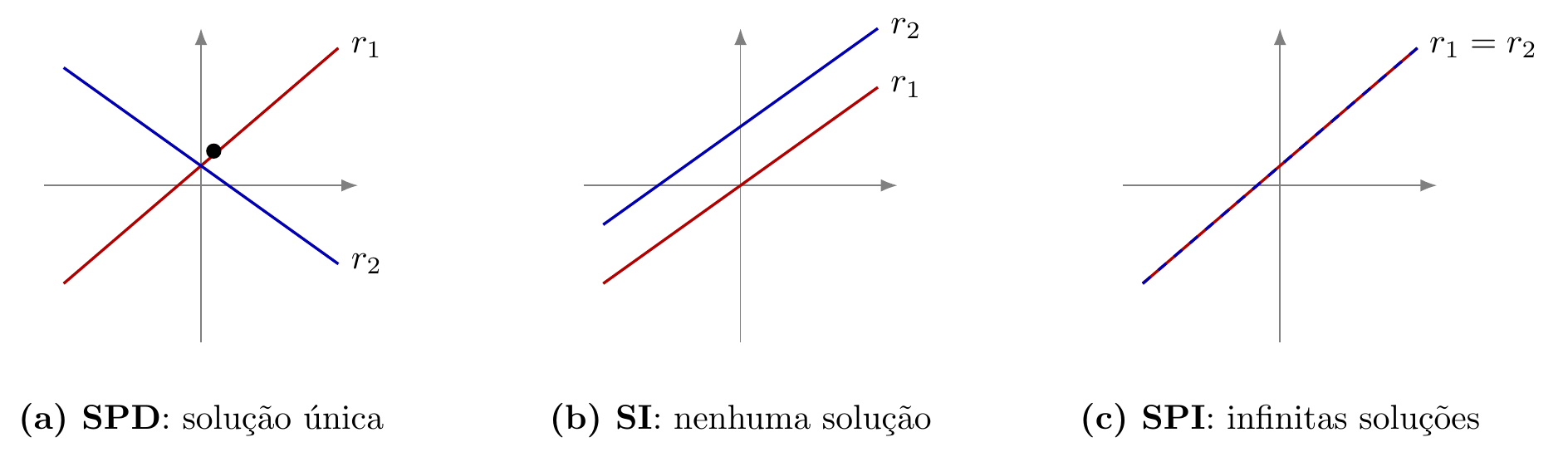
Classificação de sistemas lineares 2×2
Três painéis mostrando a interpretação geométrica de sistemas lineares 2x2 em retas: concorrentes (SPD, solução única), paralelas distintas (SI, nenhuma solução) e coincidentes (SPI, infinitas soluções).
Ver código TikZ
\begin{tikzpicture}[vec/.style={-{Latex[length=3mm]}, thick}, >=Latex]

  % ---------- Painel 1: SPD (retas concorrentes) ----------
  \begin{scope}[xshift=0cm]
    \draw[->, gray] (-1.6,0) -- (1.6,0);
    \draw[->, gray] (0,-1.6) -- (0,1.6);
    \draw[thick, red!70!black] (-1.4,-1.0) -- (1.4,1.4) node[right, black] {$r_1$};
    \draw[thick, blue!70!black] (-1.4,1.2) -- (1.4,-0.8) node[right, black] {$r_2$};
    \filldraw[black] (0.13,0.35) circle (2pt);
    \node[below=0.5cm] at (0,-1.6) {\textbf{(a) SPD}: solução única};
  \end{scope}

  % ---------- Painel 2: SI (retas paralelas distintas) ----------
  \begin{scope}[xshift=5.5cm]
    \draw[->, gray] (-1.6,0) -- (1.6,0);
    \draw[->, gray] (0,-1.6) -- (0,1.6);
    \draw[thick, red!70!black] (-1.4,-1.0) -- (1.4,1.0) node[right, black] {$r_1$};
    \draw[thick, blue!70!black] (-1.4,-0.4) -- (1.4,1.6) node[right, black] {$r_2$};
    \node[below=0.5cm] at (0,-1.6) {\textbf{(b) SI}: nenhuma solução};
  \end{scope}

  % ---------- Painel 3: SPI (retas coincidentes) ----------
  \begin{scope}[xshift=11cm]
    \draw[->, gray] (-1.6,0) -- (1.6,0);
    \draw[->, gray] (0,-1.6) -- (0,1.6);
    \draw[thick, red!70!black] (-1.4,-1.0) -- (1.4,1.4);
    \draw[thick, dashed, blue!70!black] (-1.4,-1.0) -- (1.4,1.4);
    \node[right] at (1.4,1.4) {$r_1=r_2$};
    \node[below=0.5cm] at (0,-1.6) {\textbf{(c) SPI}: infinitas soluções};
  \end{scope}

\end{tikzpicture}
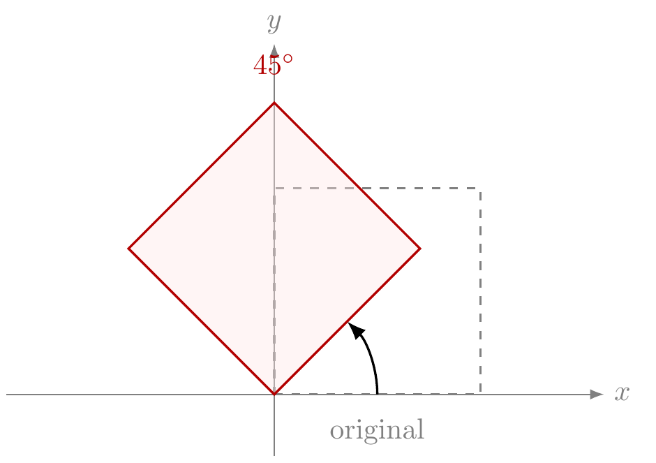
Rotação de um quadrado unitário
Quadrado unitário original (tracejado) e sua imagem sob rotação de 45° (sólido, colorido), ilustrando o efeito geométrico de uma transformação linear de rotação em R².
Ver código TikZ
\begin{tikzpicture}[scale=2.5, vec/.style={-{Latex[length=3mm]}, thick}, >=Latex]
  % axes
  \draw[gray, ->] (-1.3,0) -- (1.6,0) node[right] {$x$};
  \draw[gray, ->] (0,-0.3) -- (0,1.7) node[above] {$y$};

  % original square (dashed)
  \draw[dashed, thick, gray] (0,0) -- (1,0) -- (1,1) -- (0,1) -- cycle;
  \node[gray] at (0.5,-0.18) {original};

  % rotated square (solid, colored) by 45 degrees
  \draw[thick, red!70!black, fill=red!10, fill opacity=0.4]
    (0,0) -- (0.7071,0.7071) -- (0,1.4142) -- (-0.7071,0.7071) -- cycle;
  \node[red!70!black] at (0,1.6) {$45^\circ$};

  % angle arc
  \draw[->, thick] (0.5,0) arc (0:45:0.5);
\end{tikzpicture}