Controle Clássico
13 figura(s) nesta categoria. Fonte em figuras/controle-classico/.
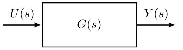
Bloco de Função de Transferência
Bloco genérico de entrada/saída G(s), com sinais U(s) e Y(s) — base para diagramas de malha de controle.
Ver código TikZ
\begin{tikzpicture}[auto, node distance=2.5cm, >=latex]
    % Estilo dos blocos
    \tikzstyle{block} = [draw, rectangle, minimum height=1.3cm, minimum width=1.4cm, line width=0.8pt]
    \tikzstyle{input} = [coordinate]
    \tikzstyle{output} = [coordinate]

    % Nós
    \node [input, name=input] {};
    \node [block, right of=input, text centered, text width=2.5cm] (system) {$G(s)$};
    \node [output, right of=system] (output) {};

    % Conexões
    \draw [draw, ->, line width=1pt] (input) -- node {$U(s)$} (system);
    \draw [draw, ->, line width=1pt] (system) -- node {$Y(s)$} (output);
\end{tikzpicture}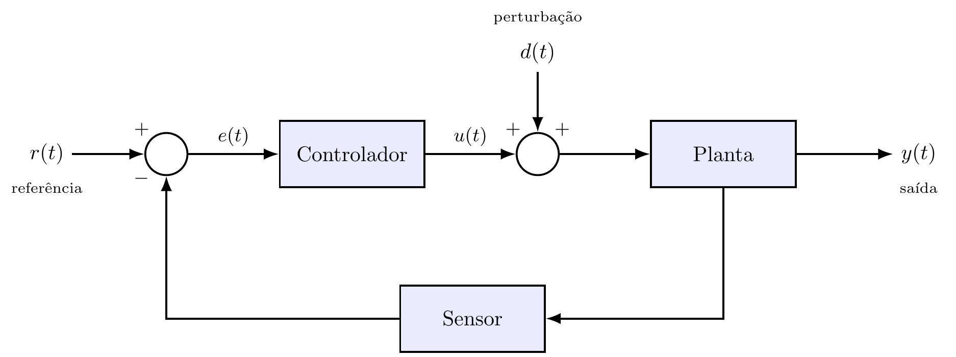
Componentes de um sistema de controle em malha fechada
Referência, erro, controlador, planta, perturbação, sensor e saída de um sistema de controle realimentado.
Ver código TikZ
% ---------------------------------------------------------------
% Componentes de um sistema de controle em malha fechada: referência,
% erro, controlador, atuador+planta, perturbação, sensor e saída.
% ---------------------------------------------------------------
\begin{tikzpicture}[>=Latex, line width=0.9pt, node distance=1.5cm,
  bloco/.style={draw, minimum width=2.4cm, minimum height=1.1cm, fill=blue!8},
  soma/.style={draw, circle, minimum size=0.7cm, inner sep=0pt},
  seta/.style={->}]

  \node (r) at (0,0) {$r(t)$};
  \node[font=\scriptsize, below=1pt of r] {referência};
  \node[soma, right=1.2cm of r]     (sum) {};
  \node[bloco, right=1.5cm of sum]  (c)   {Controlador};
  \node[soma, right=1.5cm of c]     (sum2) {};
  \node[bloco, right=1.5cm of sum2] (g)   {Planta};
  \node[right=1.6cm of g] (y) {$y(t)$};
  \node[font=\scriptsize, below=1pt of y] {saída};
  \node[bloco, below=1.6cm of c, xshift=2.0cm]  (h) {Sensor};
  \node[above=1.0cm of sum2] (d) {$d(t)$};
  \node[font=\scriptsize, above=1pt of d] {perturbação};

  \draw[seta] (r) -- (sum);
  \draw[seta] (sum) -- node[above, font=\small]{$e(t)$} (c);
  \draw[seta] (c) -- node[above, font=\small]{$u(t)$} (sum2);
  \draw[seta] (d) -- (sum2);
  \draw[seta] (sum2) -- (g);
  \draw[seta] (g) -- (y);
  \draw[seta] (g.south) |- (h.east);
  \draw[seta] (h.west) -| (sum.south);

  \node[font=\small] at ($(sum.north west)+(-0.15,0.15)$) {$+$};
  \node[font=\small] at ($(sum.south west)+(-0.15,-0.15)$) {$-$};
  \node[font=\small] at ($(sum2.north west)+(-0.15,0.15)$) {$+$};
  \node[font=\small] at ($(sum2.north east)+(0.15,0.15)$) {$+$};

\end{tikzpicture}

Sistema de controle em malha aberta
Estrutura básica de um sistema de controle em malha aberta: controlador seguido da planta, sem realimentação.

Ver código TikZ
% ---------------------------------------------------------------
% Sistema de controle em malha aberta.
% ---------------------------------------------------------------
\begin{tikzpicture}[>=Latex, line width=0.9pt, node distance=1.4cm,
  bloco/.style={draw, minimum width=2.2cm, minimum height=1.1cm, fill=blue!8},
  seta/.style={->}]

  \node (r) at (0,0) {$r(t)$};
  \node[bloco, right=of r]   (c) {Controlador};
  \node[bloco, right=of c]   (g) {Planta};
  \node[right=of g] (y) {$y(t)$};

  \draw[seta] (r) -- (c);
  \draw[seta] (c) -- node[above, font=\small]{$u(t)$} (g);
  \draw[seta] (g) -- (y);

\end{tikzpicture}
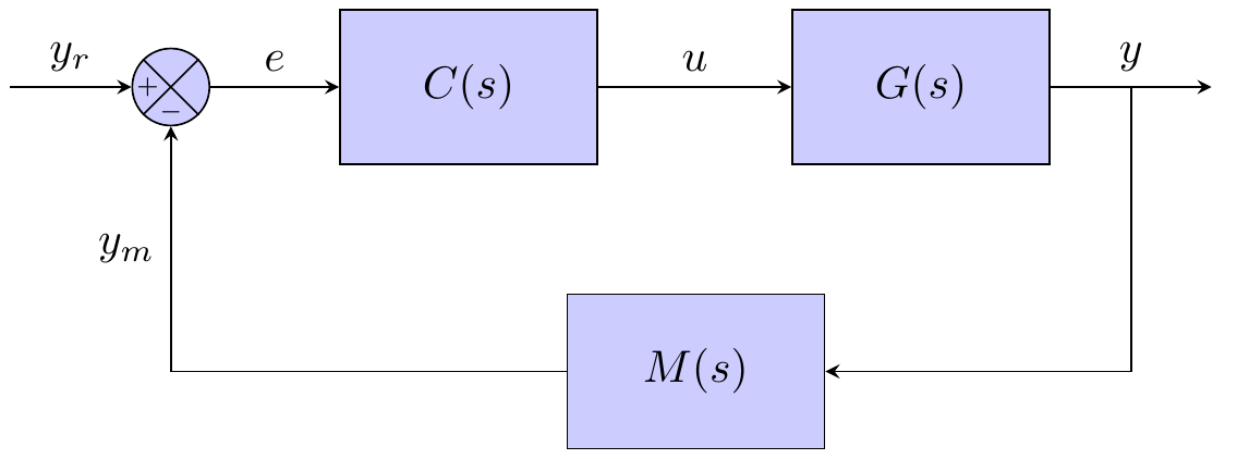
Malha de Controle Contínua (Domínio da Frequência)
Diagrama de blocos de malha fechada com controlador C(s), planta G(s) e sensor M(s), no domínio de Laplace.
Ver código TikZ
    \begin{tikzpicture}

        % Desenha o comparador:
        \node [draw, circle,
                minimum size=0.6cm,
                fill=blue!20]
              (comp) at (0,0) {};
        \draw (comp.north east) -- (comp.south west)
              (comp.north west) -- (comp.south east);
        \node [left=-1pt]
                at (comp.center){\tiny $+$};
        \node [below]
                at (comp.center){\tiny $-$};

        % Bloco do controlador:
        \node [draw,
            fill=blue!20,
            minimum width=2cm,
            minimum height=1.2cm,
            right=1cm of comp
        ]  (controlador) {$C(s)$};

        % Bloco da planta:
        \node [draw,
            fill=blue!20,
            minimum width=2cm,
            minimum height=1.2cm,
            right=1.5cm of controlador
        ] (sistema) {$G(s)$};

        % Bloco do sensor:
        \node [draw,
            fill=blue!20,
            minimum width=2cm,
            minimum height=1.2cm,
            below right= 1cm and -0.25cm of controlador
        ]  (sensor) {$M(s)$};

        % Ramos de sinais:
        % - Erro:
        \draw[-stealth] (comp.east) -- (controlador.west)
        node[midway,above]{$e$};

        % - Controle:
        \draw[-stealth] (controlador.east) -- (sistema.west)
        node[midway,above] (u) {$u$};

        % - Saída:
        \draw[-stealth] (sistema.east) -- ++ (1.25,0)
        node[midway](saida){}
        node[midway,above]{$y$};

        % - Realimentação:
        \draw[-stealth] (saida.center) |- (sensor.east);
        \draw[-stealth] (sensor.west) -| (comp.south)
        node[near end,left]{$y_m$};

        % - Referência:
        \draw[-stealth] (-1.25,0) -- (comp.west)
        node[midway,above]{$y_{r}$};

    \end{tikzpicture}

Malha de Controle Contínua (Domínio do Tempo)
Diagrama de blocos de malha fechada com controlador c(t) e planta g(t), sinais no domínio do tempo.

Ver código TikZ
\begin{tikzpicture}[
    auto,
    % Distância padrão entre os nós para compactar
    node distance=1.6cm,
    % Estilo padrão para blocos (Planta)
    block/.style={draw, fill=blue!5, rectangle, minimum height=1.2cm, minimum width=2.2cm, align=center, thick},
    % Estilo específico para o Controlador (cor diferente)
    block_ctrl/.style={draw, fill=green!5, rectangle, minimum height=1.2cm, minimum width=2.2cm, align=center, thick},
    % Estilo para o ponto de soma (menor)
    sum/.style={draw, circle, minimum size=0.5cm, thick},
    % Estilo para as setas
    arrow/.style={-Stealth, thick},
    % Ponto de derivação
    dot/.style={fill, circle, minimum size=3pt, inner sep=0pt},
    % Define o tamanho da fonte padrão para os rótulos
    every node/.style={font=\small}
]

    % --- Nós ---
    \node (input) {};
    \node [sum, right=0.8cm of input] (sum) {};

    % Controlador (domínio do tempo)
    \node [block_ctrl, right=of sum] (controller) {Controlador \\ $c(t)$};

    % Planta (domínio do tempo)
    \node [block, right=of controller] (plant) {Planta \\ $g(t)$};

    \node [right=1.8cm of plant] (output) {};

    % --- Caminho Direto ---
    \draw [arrow] (input) -- node {$r(t)$} (sum);

    \draw [arrow] (sum) -- node {$e(t)$} (controller);

    \draw [arrow] (controller) -- node {$u(t)$} (plant);

    % Posição do rótulo de saída ajustada
    \draw [arrow] (plant) -- node (y_out) [pos=0.6] {$y(t)$} (output);

    % --- Realimentação (Feedback) ---
    \node [dot, right=1.0cm of plant] (branch) {};

    % Caminho de volta
    \draw [thick] (branch) |- ++(0,-1.3) -| node[pos=0.95, xshift=0.4cm] {\textbf{--}} (sum);

    % Detalhe interno do ponto de soma (X)
    \draw (sum.north east) -- (sum.south west);
    \draw (sum.north west) -- (sum.south east);

\end{tikzpicture}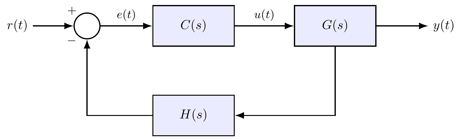
Sistema de controle em malha fechada
Sistema de controle em malha fechada com realimentação negativa unitária, C(s) e G(s).
Ver código TikZ
% ---------------------------------------------------------------
% Sistema de controle em malha fechada com realimentação negativa.
% ---------------------------------------------------------------
\begin{tikzpicture}[>=Latex, line width=0.9pt, node distance=1.6cm,
  bloco/.style={draw, minimum width=2.2cm, minimum height=1.1cm, fill=blue!8},
  soma/.style={draw, circle, minimum size=0.7cm, inner sep=0pt},
  seta/.style={->}]

  \node (r) at (0,0) {$r(t)$};
  \node[soma, right=1.1cm of r]  (sum) {};
  \node[bloco, right=1.4cm of sum] (c) {$C(s)$};
  \node[bloco, right=of c]        (g) {$G(s)$};
  \node[right=1.4cm of g] (y) {$y(t)$};
  \node[bloco, below=1.3cm of c]  (h) {$H(s)$};

  \draw[seta] (r) -- (sum);
  \draw[seta] (sum) -- node[above, font=\small]{$e(t)$} (c);
  \draw[seta] (c) -- node[above, font=\small]{$u(t)$} (g);
  \draw[seta] (g) -- (y);
  \draw[seta] (g.south) |- (h.east);
  \draw[seta] (h.west) -| (sum.south);

  \node[font=\small] at ($(sum.north west)+(-0.15,0.15)$) {$+$};
  \node[font=\small] at ($(sum.south west)+(-0.15,-0.15)$) {$-$};

\end{tikzpicture}
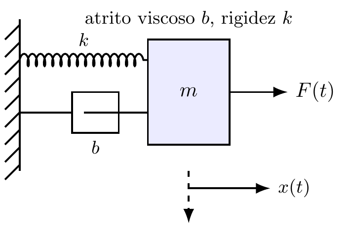
Sistema massa-mola-amortecedor
Sistema mecânico massa-mola-amortecedor com força de entrada F(t) e deslocamento x(t), exemplo clássico de modelagem.
Ver código TikZ
% ---------------------------------------------------------------
% Sistema mecânico massa-mola-amortecedor (exemplo de modelagem).
% Requer \usetikzlibrary{decorations.pathmorphing} no chunk .qmd.
% ---------------------------------------------------------------
\begin{tikzpicture}[>=Latex, line width=0.9pt]

  % parede
  \draw (0,-1.0) -- (0,1.6);
  \foreach \y in {-0.9,-0.6,...,1.5}
    \draw (0,\y) -- (-0.25,\y-0.25);

  % mola
  \draw[decorate, decoration={coil, aspect=0.4, segment length=4pt, amplitude=3pt}]
    (0,0.9) -- (2.2,0.9);
  \node[font=\small] at (1.1,1.25) {$k$};

  % amortecedor
  \draw (0,0.0) -- (0.9,0.0);
  \draw (0.9,-0.35) rectangle (1.7,0.35);
  \draw (1.1,0.0) -- (2.2,0.0);
  \node[font=\small] at (1.3,-0.6) {$b$};

  % massa
  \draw[fill=blue!8] (2.2,-0.55) rectangle (3.6,1.25);
  \node at (2.9,0.35) {$m$};

  % força e deslocamento
  \draw[->] (3.6,0.35) -- (4.6,0.35) node[right] {$F(t)$};
  \draw[->, dashed] (2.9,-1.0) -- (2.9,-1.9) node[below]{};
  \draw[->] (2.9,-1.3) -- (4.3,-1.3) node[right, font=\small] {$x(t)$};

  \node[font=\small] at (2.9,1.6) {atrito viscoso $b$, rigidez $k$};

\end{tikzpicture}
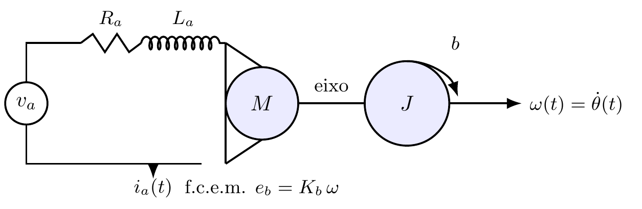
Motor CC controlado pela armadura
Circuito elétrico de armadura do motor CC acoplado à carga mecânica, exemplo de modelagem eletromecânica.
Ver código TikZ
% ---------------------------------------------------------------
% Motor CC controlado pela armadura — circuito elétrico + carga
% mecânica (exemplo de modelagem eletromecânica).
% Requer \usetikzlibrary{decorations.pathmorphing} no chunk .qmd.
% ---------------------------------------------------------------
\begin{tikzpicture}[>=Latex, line width=0.9pt]

  % fonte de tensão de armadura
  \draw (0,0) circle (0.35);
  \node at (0,0) {$v_a$};
  \draw (0,0.35) -- (0,1.0) -- (0.9,1.0);
  \draw (0,-0.35) -- (0,-1.0) -- (2.9,-1.0);

  % resistor de armadura Ra (zigzag manual)
  \draw (0.9,1.0) -- (1.1,1.15) -- (1.3,0.85) -- (1.5,1.15) -- (1.7,0.85) -- (1.9,1.0);
  \node[font=\small] at (1.4,1.4) {$R_a$};

  % indutor de armadura La
  \draw[decorate, decoration={coil, aspect=0.5, segment length=4pt, amplitude=3pt}]
    (1.9,1.0) -- (3.3,1.0);
  \node[font=\small] at (2.6,1.4) {$L_a$};

  % motor (rotor)
  \draw[fill=blue!8] (3.3,1.0) -- (3.3,-1.0) arc (180:-180:0.0);
  \draw[fill=blue!8] (3.9,0.0) circle (0.6);
  \node at (3.9,0.0) {$M$};
  \draw (3.3,1.0) -- (3.9,0.6);
  \draw (3.3,-1.0) -- (3.9,-0.6);
  \node[font=\small] at (3.9,-1.4) {f.c.e.m. $e_b = K_b\,\omega$};

  % eixo
  \draw (4.5,0.0) -- (5.6,0.0);
  \node[font=\small] at (5.05,0.3) {eixo};

  % carga mecânica: inércia J e atrito b
  \draw[fill=blue!8] (6.3,0.0) circle (0.7);
  \node at (6.3,0.0) {$J$};
  \draw[->] (6.3,0.7) arc (90:20:0.9);
  \node[font=\small] at (7.1,1.0) {$b$};

  \draw[->] (7.0,0.0) -- (8.2,0.0) node[right, font=\small] {$\omega(t) = \dot\theta(t)$};

  \node[font=\small] at (2.1,-1.4) {$i_a(t)$};
  \draw[->] (2.1,-1.0) -- (2.1,-1.25);

\end{tikzpicture}
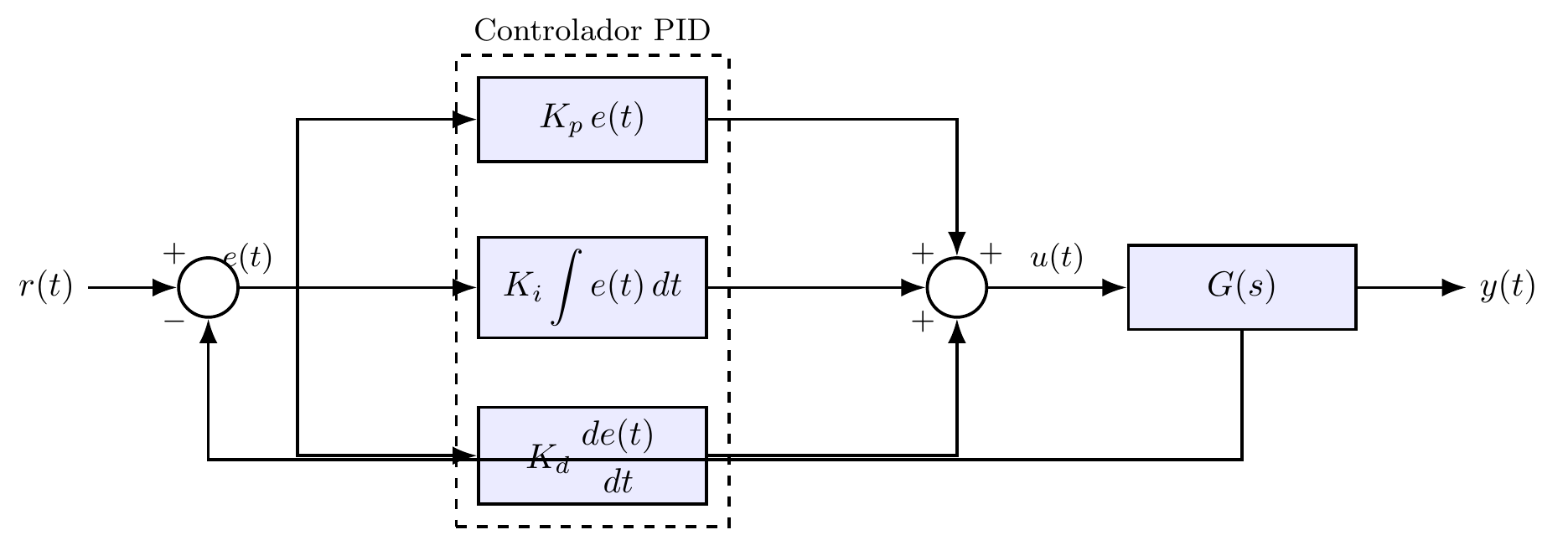
Bloco PID em malha fechada
Estrutura interna do controlador PID (proporcional, integral e derivativo) atuando em malha fechada sobre uma planta G(s).
Ver código TikZ
% ---------------------------------------------------------------
% Estrutura interna do controlador PID em malha fechada.
% ---------------------------------------------------------------
\begin{tikzpicture}[>=Latex, line width=0.9pt, node distance=1.0cm,
  bloco/.style={draw, minimum width=2.3cm, minimum height=0.85cm, fill=blue!8},
  soma/.style={draw, circle, minimum size=0.6cm, inner sep=0pt},
  seta/.style={->}]

  \node (r) at (0,0) {$r(t)$};
  \node[soma, right=0.9cm of r] (s1) {};

  \node[bloco, right=2.4cm of s1, yshift=1.7cm]  (p) {$K_p\,e(t)$};
  \node[bloco, right=2.4cm of s1]                (i) {$K_i\displaystyle\int e(t)\,dt$};
  \node[bloco, right=2.4cm of s1, yshift=-1.7cm] (d) {$K_d\,\dfrac{de(t)}{dt}$};

  \node[soma, right=2.2cm of i] (s2) {};
  \node[bloco, right=1.4cm of s2] (g) {$G(s)$};
  \node[right=1.1cm of g] (y) {$y(t)$};

  \draw[seta] (r) -- (s1);
  \draw[seta] (s1) -- node[above, font=\small, pos=0.15]{$e(t)$} ++(0.9,0) |- (p.west);
  \draw[seta] (s1) -- (i.west);
  \draw[seta] (s1) -- ++(0.9,0) |- (d.west);

  \draw[seta] (p.east) -| (s2.north);
  \draw[seta] (i.east) -- (s2);
  \draw[seta] (d.east) -| (s2.south);

  \draw[seta] (s2) -- node[above, font=\small]{$u(t)$} (g);
  \draw[seta] (g) -- (y);
  \draw[seta] (g.south) |- ++(0,-1.3) -| (s1.south);

  \node[font=\small] at ($(s1.north west)+(-0.12,0.12)$) {$+$};
  \node[font=\small] at ($(s1.south west)+(-0.12,-0.12)$) {$-$};
  \node[font=\small] at ($(s2.north west)+(-0.12,0.12)$) {$+$};
  \node[font=\small] at ($(s2.south west)+(-0.12,-0.12)$) {$+$};
  \node[font=\small] at ($(s2.north east)+(0.12,0.12)$) {$+$};

  \node[font=\small, draw, dashed, fit=(p)(i)(d), inner sep=6pt, label={[font=\small]above:Controlador PID}] {};

\end{tikzpicture}

Álgebra de blocos: associação em paralelo
Redução de dois blocos G1(s) e G2(s) em paralelo para um único bloco equivalente G1(s)+G2(s).

Ver código TikZ
% ---------------------------------------------------------------
% Álgebra de blocos: associação em paralelo.
% ---------------------------------------------------------------
\begin{tikzpicture}[>=Latex, line width=0.9pt, node distance=1.3cm,
  bloco/.style={draw, minimum width=1.8cm, minimum height=1.0cm, fill=blue!8},
  soma/.style={draw, circle, minimum size=0.6cm, inner sep=0pt},
  seta/.style={->}]

  \node (x) at (0,0) {$X(s)$};
  \coordinate (bx) at (1.0,0);
  \node[bloco, right=1.9cm of x, yshift=0.9cm]  (g1) {$G_1(s)$};
  \node[bloco, right=1.9cm of x, yshift=-0.9cm] (g2) {$G_2(s)$};
  \node[soma, right=4.6cm of x] (sum) {};
  \node[right=0.9cm of sum] (y) {$Y(s)$};

  \draw[seta] (x) -- (bx);
  \draw[seta] (bx) |- (g1.west);
  \draw[seta] (bx) |- (g2.west);
  \draw[seta] (g1.east) -| (sum.north);
  \draw[seta] (g2.east) -| (sum.south);
  \draw[seta] (sum) -- (y);
  \node[font=\small] at ($(sum.north west)+(-0.12,0.12)$) {$+$};
  \node[font=\small] at ($(sum.south west)+(-0.12,-0.12)$) {$+$};

  \node[font=\Large, right=1.1cm of y] (eq) {$\equiv$};

  \node[right=1.1cm of eq] (x2) {$X(s)$};
  \node[bloco, right=of x2, minimum width=2.8cm] (geq) {$G_1(s)+G_2(s)$};
  \node[right=of geq] (y2) {$Y(s)$};
  \draw[seta] (x2) -- (geq);
  \draw[seta] (geq) -- (y2);

\end{tikzpicture}

Álgebra de blocos: redução de realimentação negativa
Redução de uma malha de realimentação negativa para o bloco equivalente G(s)/(1+G(s)H(s)).

Ver código TikZ
% ---------------------------------------------------------------
% Álgebra de blocos: redução de uma malha de realimentação negativa.
% ---------------------------------------------------------------
\begin{tikzpicture}[>=Latex, line width=0.9pt, node distance=1.3cm,
  bloco/.style={draw, minimum width=1.8cm, minimum height=1.0cm, fill=blue!8},
  soma/.style={draw, circle, minimum size=0.6cm, inner sep=0pt},
  seta/.style={->}]

  \node (x) at (0,0) {$X(s)$};
  \node[soma, right=1.0cm of x] (sum) {};
  \node[bloco, right=1.1cm of sum] (g) {$G(s)$};
  \node[right=1.0cm of g] (y) {$Y(s)$};
  \node[bloco, below=0.9cm of g] (h) {$H(s)$};

  \draw[seta] (x) -- (sum);
  \draw[seta] (sum) -- (g);
  \draw[seta] (g) -- (y);
  \draw[seta] (g.south) -- (h.north);
  \draw[seta] (h.west) -| (sum.south);
  \node[font=\small] at ($(sum.north west)+(-0.12,0.12)$) {$+$};
  \node[font=\small] at ($(sum.south west)+(-0.12,-0.12)$) {$-$};

  \node[font=\Large, right=1.1cm of y] (eq) {$\equiv$};

  \node[right=1.1cm of eq] (x2) {$X(s)$};
  \node[bloco, right=of x2, minimum width=3.2cm] (geq) {$\dfrac{G(s)}{1+G(s)H(s)}$};
  \node[right=of geq] (y2) {$Y(s)$};
  \draw[seta] (x2) -- (geq);
  \draw[seta] (geq) -- (y2);

\end{tikzpicture}
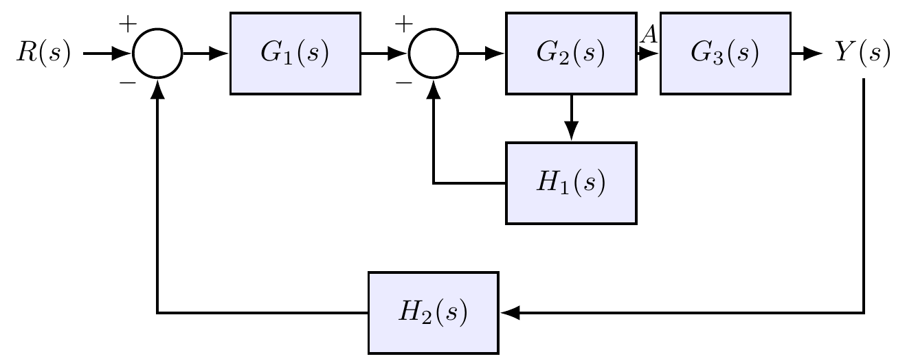
Exemplo de redução por álgebra de blocos
Diagrama de blocos com múltiplas malhas aninhadas, para exercício de redução por álgebra de blocos ou regra de Mason.
Ver código TikZ
% ---------------------------------------------------------------
% Exemplo de diagrama de blocos com múltiplas malhas, para exercício
% de redução por álgebra de blocos / regra de Mason.
% ---------------------------------------------------------------
\begin{tikzpicture}[>=Latex, line width=0.9pt,
  bloco/.style={draw, minimum width=1.6cm, minimum height=1.0cm, fill=blue!8},
  soma/.style={draw, circle, minimum size=0.6cm, inner sep=0pt},
  seta/.style={->}]

  % --- caminho direto (y = 0) ---
  \node (r)  at (0,0)    {$R(s)$};
  \node[soma]  (s1) at (1.4,0)  {};
  \node[bloco] (g1) at (3.1,0)  {$G_1(s)$};
  \node[soma]  (s2) at (4.8,0)  {};
  \node[bloco] (g2) at (6.5,0)  {$G_2(s)$};
  \node[bloco] (g3) at (8.4,0)  {$G_3(s)$};
  \node (y)  at (10.1,0) {$Y(s)$};

  \draw[seta] (r)  -- (s1);
  \draw[seta] (s1) -- (g1);
  \draw[seta] (g1) -- (s2);
  \draw[seta] (s2) -- (g2);
  \draw[seta] (g2) -- node[above, font=\small]{$A$} (g3);
  \draw[seta] (g3) -- (y);

  % --- malha interna: H1 realimenta de A (saída de G2) para s2 ---
  \node[bloco] (h1) at (6.5,-1.6) {$H_1(s)$};
  \draw[seta] (g2.south) -- (h1.north);
  \draw[seta] (h1.west) -| (s2.south);

  % --- malha externa: H2 realimenta de Y para s1 ---
  \node[bloco] (h2) at (4.8,-3.2) {$H_2(s)$};
  \draw[seta] (y.south) |- (h2.east);
  \draw[seta] (h2.west) -| (s1.south);

  \node[font=\small] at ($(s1.north west)+(-0.14,0.14)$) {$+$};
  \node[font=\small] at ($(s1.south west)+(-0.14,-0.14)$) {$-$};
  \node[font=\small] at ($(s2.north west)+(-0.14,0.14)$) {$+$};
  \node[font=\small] at ($(s2.south west)+(-0.14,-0.14)$) {$-$};

\end{tikzpicture}

Álgebra de blocos: associação em série
Redução de dois blocos G1(s) e G2(s) em cascata (série) para um único bloco equivalente G1(s)G2(s).

Ver código TikZ
% ---------------------------------------------------------------
% Álgebra de blocos: associação em série (cascata).
% ---------------------------------------------------------------
\begin{tikzpicture}[>=Latex, line width=0.9pt, node distance=1.3cm,
  bloco/.style={draw, minimum width=1.8cm, minimum height=1.0cm, fill=blue!8},
  seta/.style={->}]

  \node (x) at (0,0) {$X(s)$};
  \node[bloco, right=of x] (g1) {$G_1(s)$};
  \node[bloco, right=of g1] (g2) {$G_2(s)$};
  \node[right=of g2] (y) {$Y(s)$};
  \draw[seta] (x) -- (g1);
  \draw[seta] (g1) -- (g2);
  \draw[seta] (g2) -- (y);

  \node[font=\Large, right=1.1cm of y] (eq) {$\equiv$};

  \node[right=1.1cm of eq] (x2) {$X(s)$};
  \node[bloco, right=of x2, minimum width=2.6cm] (geq) {$G_1(s)\,G_2(s)$};
  \node[right=of geq] (y2) {$Y(s)$};
  \draw[seta] (x2) -- (geq);
  \draw[seta] (geq) -- (y2);

\end{tikzpicture}