Circuitos CA
14 figura(s) nesta categoria. Fonte em figuras/circuitos-ca/.
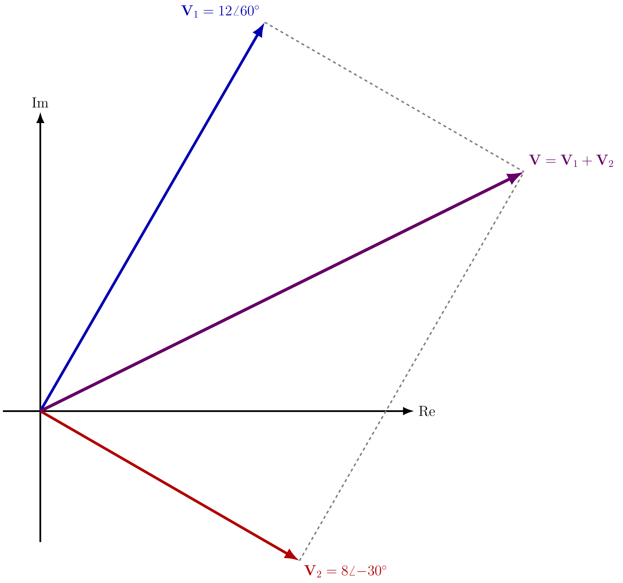
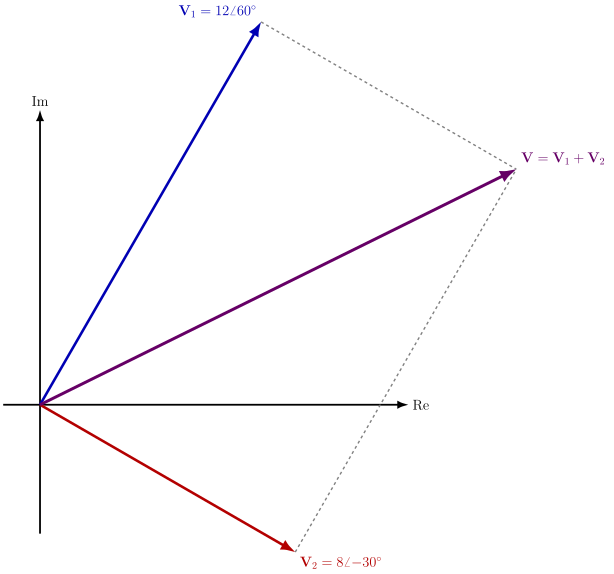
Adição de fasores (regra do paralelogramo)
Soma vetorial de dois fasores no plano complexo pela regra do paralelogramo (V = V1 + V2).
Ver código TikZ
% ---------------------------------------------------------------------
% Adição de fasores pela regra do paralelogramo.
% V1 = 12∠60°, V2 = 8∠-30°, V = V1 + V2
% ---------------------------------------------------------------------
\begin{tikzpicture}[>=Latex, line width=1.8pt, font=\Large, scale=1.3]

  \draw[->] (-1,0) -- (10,0) node[right] {Re};
  \draw[->] (0,-3.5) -- (0,8) node[above] {Im};

  \coordinate (V1) at ({12*cos(60)},{12*sin(60)});
  \coordinate (V2) at ({8*cos(-30)},{8*sin(-30)});
  \coordinate (V)  at ($(V1)+(V2)$);

  \draw[->, blue!70!black, line width=2.6pt] (0,0) -- (V1)
    node[above left] {$\mathbf{V}_1 = 12\angle 60^\circ$};
  \draw[->, red!70!black, line width=2.6pt] (0,0) -- (V2)
    node[below right] {$\mathbf{V}_2 = 8\angle{-30^\circ}$};
  \draw[->, violet!80!black, line width=3pt] (0,0) -- (V)
    node[above right] {$\mathbf{V} = \mathbf{V}_1+\mathbf{V}_2$};

  \draw[dashed, gray, line width=1.4pt] (V1) -- (V);
  \draw[dashed, gray, line width=1.4pt] (V2) -- (V);

\end{tikzpicture}
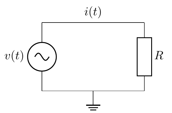
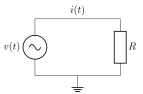
Circuito CA Simples com Carga Resistiva
Fonte de tensão senoidal v(t) alimentando uma carga resistiva R, com corrente i(t) e referência de terra.
Ver código TikZ
\begin{tikzpicture}
  % Coordenadas
  \coordinate (A) at (0,2);
  \coordinate (B) at (3,2);
  \coordinate (C) at (3,0);
  \coordinate (D) at (0,0);

  % Fonte de tensão CA
  \draw (D) to[vsourcesin, l=$v(t)$] (A);

  % Fio superior com apenas o rótulo i(t) (sem seta)
  \draw (A) -- (B) node[midway, above] {$i(t)$};

  % Carga (retângulo)
  \draw (B) to[generic, l=$R$] (C);

  % Fio inferior com referência no ponto médio
  \draw (C) -- (D);
  \draw ($(C)!0.5!(D)$) node[ground]{};

\end{tikzpicture}
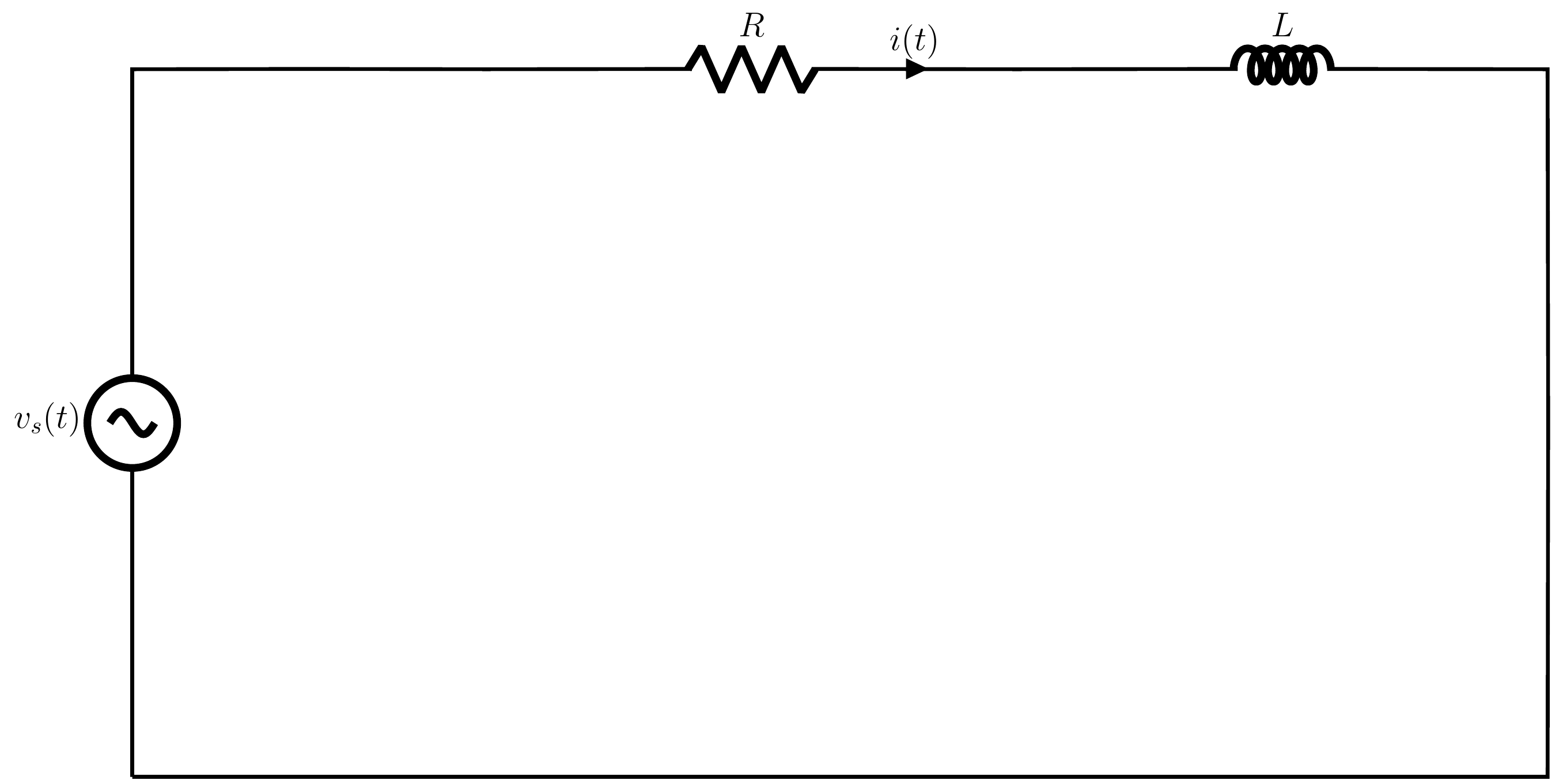
Circuito RL série
Circuito RL série alimentado por fonte de tensão senoidal, com a corrente i(t) em destaque.
Ver código TikZ
% ---------------------------------------------------------------------
% Circuito RL série alimentado por fonte senoidal.
% Requer circuitikz (habilitado via engine.opts na aula).
% ---------------------------------------------------------------------
\ctikzset{bipoles/length=2.2cm}
\begin{circuitikz}[scale=2.6, line width=1.6pt, font=\Large]
\draw (0,0)
  to[sinusoidal voltage source, l=$v_s(t)$] (0,4)
  to[short] (2,4)
  to[R=$R$, i=$i(t)$] (5,4)
  to[L=$L$] (8,4)
  to[short] (8,0)
  to[short] (0,0);
\end{circuitikz}
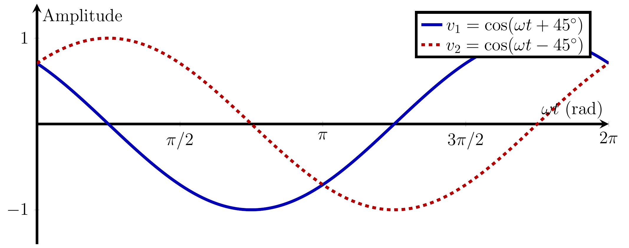
Defasagem entre senoides
Duas senoides de mesma frequência com fases diferentes, ilustrando o conceito de defasagem.
Ver código TikZ
% ---------------------------------------------------------------------
% Duas senoides de mesma frequência com fases diferentes (defasagem).
% Requer pgfplots (habilitado via engine.opts na aula).
% ---------------------------------------------------------------------
\begin{tikzpicture}
\begin{axis}[
  width=18cm, height=8.5cm,
  axis lines=middle,
  label style={font=\Large},
  tick label style={font=\Large},
  xlabel={$\omega t$ (rad)}, ylabel={Amplitude},
  xtick={0,90,180,270,360},
  xticklabels={$0$,$\pi/2$,$\pi$,$3\pi/2$,$2\pi$},
  ytick={-1,0,1},
  ymin=-1.4, ymax=1.4,
  xmin=0, xmax=360,
  domain=0:360, samples=200,
  enlargelimits=false,
  legend pos=north east,
  legend style={font=\Large},
  line width=2.2pt,
]
\addplot[blue!70!black, line width=2.4pt] {cos(x+45)};
\addlegendentry{$v_1 = \cos(\omega t + 45^\circ)$}
\addplot[red!70!black, line width=2.4pt, dashed] {cos(x-45)};
\addlegendentry{$v_2 = \cos(\omega t - 45^\circ)$}
\end{axis}
\end{tikzpicture}
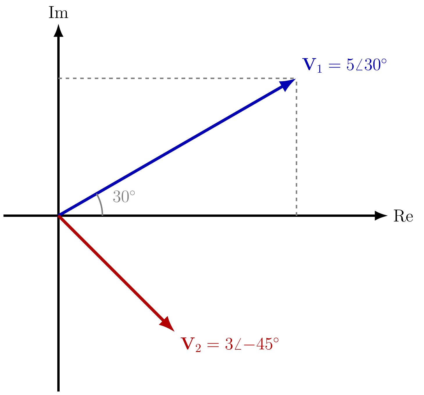
Diagrama fasorial
Dois fasores no plano complexo (V1 = 5∠30°, V2 = 3∠-45°) com projeções e ângulo destacados.
Ver código TikZ
% ---------------------------------------------------------------------
% Diagrama fasorial: dois fasores no plano complexo.
% V1 = 5∠30°, V2 = 3∠-45°
% ---------------------------------------------------------------------
\begin{tikzpicture}[>=Latex, line width=1.8pt, font=\Large, scale=1.6]

  \draw[->] (-1,0) -- (6,0) node[right] {Re};
  \draw[->] (0,-3.2) -- (0,3.5) node[above] {Im};

  \draw[->, blue!70!black, line width=2.4pt]
    (0,0) -- ({5*cos(30)},{5*sin(30)})
    node[above right] {$\mathbf{V}_1 = 5\angle 30^\circ$};

  \draw[->, red!70!black, line width=2.4pt]
    (0,0) -- ({3*cos(-45)},{3*sin(-45)})
    node[below right] {$\mathbf{V}_2 = 3\angle{-45^\circ}$};

  \draw[dashed, gray, line width=1.2pt] ({5*cos(30)},0) -- ({5*cos(30)},{5*sin(30)});
  \draw[dashed, gray, line width=1.2pt] (0,{5*sin(30)}) -- ({5*cos(30)},{5*sin(30)});

  \draw[gray, line width=1.2pt] (0.8,0) arc (0:30:0.8);
  \node[gray] at (1.2,0.35) {$30^\circ$};

\end{tikzpicture}
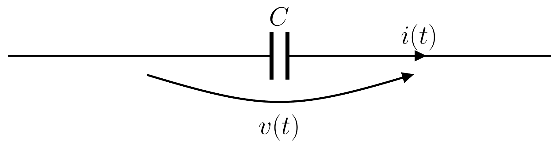
Capacitor com referências de tensão e corrente
Elemento capacitor com as referências de tensão v(t) e corrente i(t) indicadas.
Ver código TikZ
% ---------------------------------------------------------------------
% Capacitor com referências de tensão e corrente.
% Requer circuitikz (habilitado via engine.opts na aula).
% ---------------------------------------------------------------------
\ctikzset{bipoles/length=2.2cm}
\begin{circuitikz}[scale=3, line width=1.6pt, font=\huge]
\draw (0,0) to[C=$C$, i=$i(t)$, v=$v(t)$] (5,0);
\end{circuitikz}

Indutor com referências de tensão e corrente
Elemento indutor com as referências de tensão v(t) e corrente i(t) indicadas.

Ver código TikZ
% ---------------------------------------------------------------------
% Indutor com referências de tensão e corrente.
% Requer circuitikz (habilitado via engine.opts na aula).
% ---------------------------------------------------------------------
\ctikzset{bipoles/length=2.2cm}
\begin{circuitikz}[scale=3, line width=1.6pt, font=\huge]
\draw (0,0) to[L=$L$, i=$i(t)$, v=$v(t)$] (5,0);
\end{circuitikz}
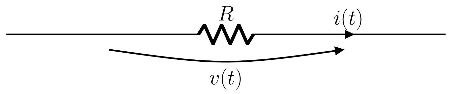
Resistor com referências de tensão e corrente
Elemento resistor com as referências de tensão v(t) e corrente i(t) indicadas.
Ver código TikZ
% ---------------------------------------------------------------------
% Resistor com referências de tensão e corrente.
% Requer circuitikz (habilitado via engine.opts na aula).
% ---------------------------------------------------------------------
\ctikzset{bipoles/length=2.2cm}
\begin{circuitikz}[scale=3, line width=1.6pt, font=\huge]
\draw (0,0) to[R=$R$, i=$i(t)$, v=$v(t)$] (5,0);
\end{circuitikz}
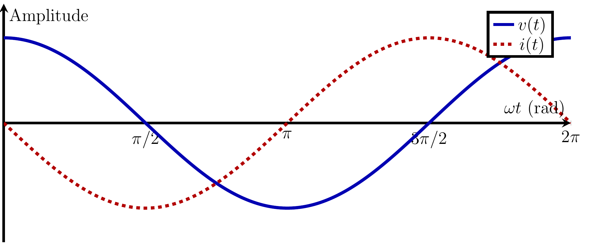
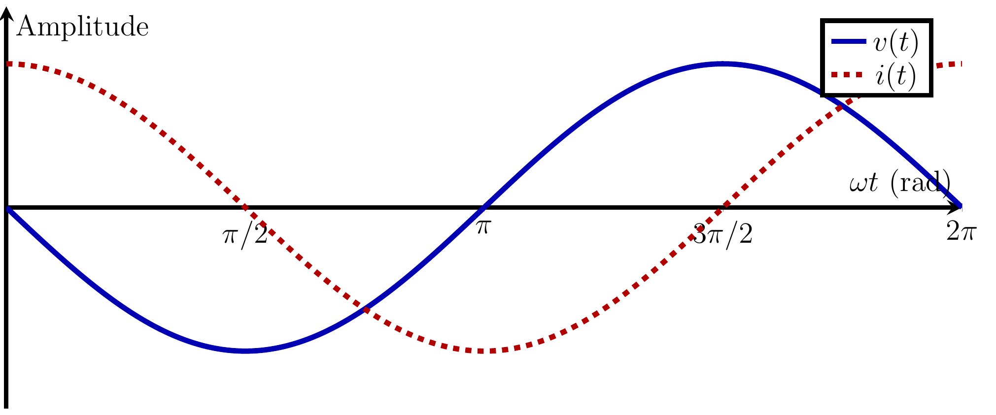
Relação de fase do capacitor
A corrente i(t) adianta a tensão v(t) em 90° num capacitor.
Ver código TikZ
% ---------------------------------------------------------------------
% Capacitor: i(t) adianta v(t) em 90°.
% Requer pgfplots (habilitado via engine.opts na aula).
% ---------------------------------------------------------------------
\begin{tikzpicture}
\begin{axis}[
  width=18cm, height=8.5cm,
  axis lines=middle,
  label style={font=\Large},
  tick label style={font=\Large},
  xlabel={$\omega t$ (rad)}, ylabel={Amplitude},
  xtick={0,90,180,270,360},
  xticklabels={$0$,$\pi/2$,$\pi$,$3\pi/2$,$2\pi$},
  ytick=\empty,
  ymin=-1.4, ymax=1.4,
  xmin=0, xmax=360,
  domain=0:360, samples=200,
  enlargelimits=false,
  legend pos=north east,
  legend style={font=\Large},
  line width=2.2pt,
]
\addplot[blue!70!black, line width=2.6pt] {cos(x)};
\addlegendentry{$v(t)$}
\addplot[red!70!black, line width=2.6pt, dashed] {cos(x+90)};
\addlegendentry{$i(t)$}
\end{axis}
\end{tikzpicture}
Relação de fase do indutor
A tensão v(t) adianta a corrente i(t) em 90° num indutor.
Ver código TikZ
% ---------------------------------------------------------------------
% Indutor: v(t) adianta i(t) em 90°.
% Requer pgfplots (habilitado via engine.opts na aula).
% ---------------------------------------------------------------------
\begin{tikzpicture}
\begin{axis}[
  width=18cm, height=8.5cm,
  axis lines=middle,
  label style={font=\Large},
  tick label style={font=\Large},
  xlabel={$\omega t$ (rad)}, ylabel={Amplitude},
  xtick={0,90,180,270,360},
  xticklabels={$0$,$\pi/2$,$\pi$,$3\pi/2$,$2\pi$},
  ytick=\empty,
  ymin=-1.4, ymax=1.4,
  xmin=0, xmax=360,
  domain=0:360, samples=200,
  enlargelimits=false,
  legend pos=north east,
  legend style={font=\Large},
  line width=2.2pt,
]
\addplot[blue!70!black, line width=2.6pt] {cos(x+90)};
\addlegendentry{$v(t)$}
\addplot[red!70!black, line width=2.6pt, dashed] {cos(x)};
\addlegendentry{$i(t)$}
\end{axis}
\end{tikzpicture}
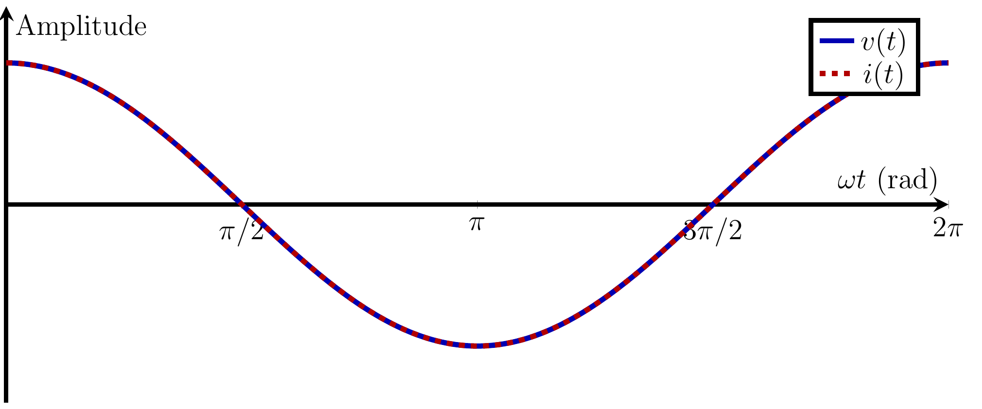
Relação de fase do resistor
Tensão v(t) e corrente i(t) em fase num resistor.
Ver código TikZ
% ---------------------------------------------------------------------
% Resistor: v(t) e i(t) em fase.
% Requer pgfplots (habilitado via engine.opts na aula).
% ---------------------------------------------------------------------
\begin{tikzpicture}
\begin{axis}[
  width=18cm, height=8.5cm,
  axis lines=middle,
  label style={font=\Large},
  tick label style={font=\Large},
  xlabel={$\omega t$ (rad)}, ylabel={Amplitude},
  xtick={0,90,180,270,360},
  xticklabels={$0$,$\pi/2$,$\pi$,$3\pi/2$,$2\pi$},
  ytick=\empty,
  ymin=-1.4, ymax=1.4,
  xmin=0, xmax=360,
  domain=0:360, samples=200,
  enlargelimits=false,
  legend pos=north east,
  legend style={font=\Large},
  line width=2.2pt,
]
\addplot[blue!70!black, line width=2.6pt] {cos(x)};
\addlegendentry{$v(t)$}
\addplot[red!70!black, line width=2.6pt, dashed] {cos(x)};
\addlegendentry{$i(t)$}
\end{axis}
\end{tikzpicture}
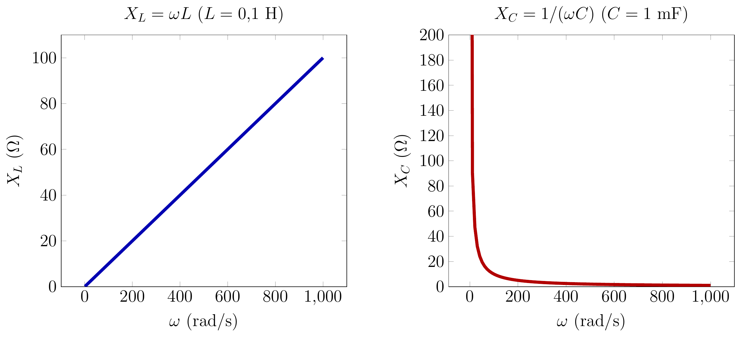
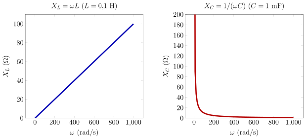
Reatâncias indutiva e capacitiva
Reatância indutiva X_L=wL e capacitiva X_C=1/(wC) em função da frequência angular.
Ver código TikZ
% ---------------------------------------------------------------------
% Reatância indutiva X_L = wL e capacitiva X_C = 1/(wC) versus frequência.
% Requer pgfplots + biblioteca groupplots (usetikzlibrary/usepgfplotslibrary
% no chunk que faz o \input).
% ---------------------------------------------------------------------
\begin{tikzpicture}
\begin{groupplot}[
  group style={group size=2 by 1, horizontal sep=3cm},
  width=10cm, height=9cm,
  label style={font=\Large},
  tick label style={font=\Large},
  title style={font=\Large},
  ymin=0,
]
\nextgroupplot[
  xlabel={$\omega$ (rad/s)}, ylabel={$X_L$ ($\Omega$)},
  title={$X_L = \omega L$ ($L=0{,}1$ H)},
  domain=1:1000, samples=100,
]
\addplot[blue!70!black, line width=2.6pt] {0.1*x};

\nextgroupplot[
  xlabel={$\omega$ (rad/s)}, ylabel={$X_C$ ($\Omega$)},
  title={$X_C = 1/(\omega C)$ ($C=1$ mF)},
  domain=1:1000, samples=100,
  ymax=200,
]
\addplot[red!70!black, line width=2.6pt] {1/(0.001*x)};
\end{groupplot}
\end{tikzpicture}
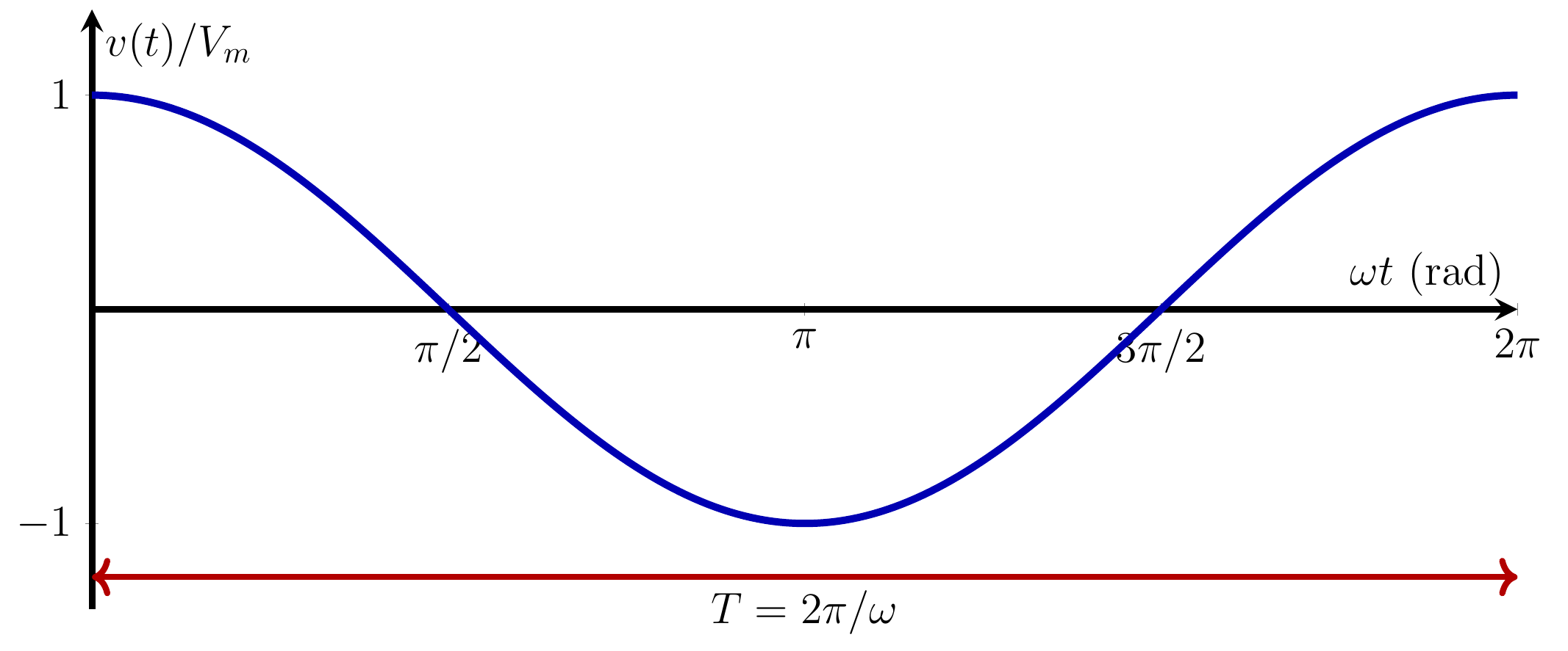
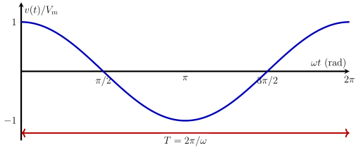
Sinal senoidal básico
Sinal senoidal v(t)=cos(wt) com o período T em destaque.
Ver código TikZ
% ---------------------------------------------------------------------
% Sinal senoidal v(t) = cos(omega t), com o período T em destaque.
% Requer pgfplots (habilitado via engine.opts na aula).
% ---------------------------------------------------------------------
\begin{tikzpicture}
\begin{axis}[
  width=18cm, height=8.5cm,
  axis lines=middle,
  label style={font=\Large},
  tick label style={font=\Large},
  xlabel={$\omega t$ (rad)}, ylabel={$v(t)/V_m$},
  xtick={0,90,180,270,360},
  xticklabels={$0$,$\pi/2$,$\pi$,$3\pi/2$,$2\pi$},
  ytick={-1,0,1},
  ymin=-1.4, ymax=1.4,
  xmin=0, xmax=360,
  domain=0:360, samples=200,
  enlargelimits=false,
  clip=false,
  line width=2.2pt,
]
\addplot[blue!70!black, line width=2.4pt] {cos(x)};
\draw[red!70!black, <->, line width=2pt] (axis cs:0,-1.25) -- (axis cs:360,-1.25)
  node[midway, below, font=\Large, black, fill=white] {$T = 2\pi/\omega$};
\end{axis}
\end{tikzpicture}

Sistema de geração, transmissão e distribuição em CA
Diagrama de blocos do sistema elétrico de potência: geração, elevação de tensão, transmissão, abaixamento e carga.

Ver código TikZ
% ---------------------------------------------------------------------
% Sistema de geração, transmissão e distribuição de energia em CA.
% ---------------------------------------------------------------------
\begin{tikzpicture}[>=Latex, line width=1.6pt, font=\Large,
  bloco/.style={draw, line width=1.6pt, minimum width=3.6cm, minimum height=1.9cm,
                fill=blue!8, align=center}]

  \node[bloco] (ger)  at (0,0)   {Geração\\60\,Hz};
  \node[bloco] (elev) at (4.8,0) {Elevação\\de tensão};
  \node[bloco] (lt)   at (9.6,0) {Linha de\\transmissão};
  \node[bloco] (abx)  at (14.4,0) {Abaixamento\\de tensão};
  \node[bloco] (carga) at (19.2,0) {Carga};

  \draw[->] (ger)  -- (elev);
  \draw[->] (elev) -- (lt);
  \draw[->] (lt)   -- (abx);
  \draw[->] (abx)  -- (carga);

  \node[font=\Large] at (0,-1.7)    {baixa tensão};
  \node[font=\Large] at (9.6,-1.7)  {alta tensão};
  \node[font=\Large] at (19.2,-1.7) {baixa tensão};

\end{tikzpicture}