Controle por Espaço de Estados
12 figura(s) nesta categoria. Fonte em figuras/controle-estados/.
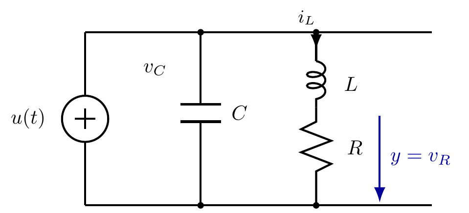
Circuito RLC em espaço de estados
Circuito RLC com fonte u(t), cujas equações de estado (tensão no capacitor e corrente no indutor) modelam a dinâmica do sistema.
Ver código TikZ
% ---------------------------------------------------------------
% Circuito RLC:  u(t) em paralelo com C  e  com o ramo série L–R
%   C dvC/dt = u - iL ;  L diL/dt = vC - R iL ;  y = vR = R iL
% Bibliotecas (carregadas no chunk .qmd):
%   arrows.meta, positioning, calc, decorations.pathmorphing
% ---------------------------------------------------------------
\begin{tikzpicture}[>=Latex, line width=1pt]

  % --- Trilhos ---
  \draw (0,0) -- (6,0);
  \draw (0,3) -- (6,3);

  % --- Fonte u(t) ---
  \draw (0,0) -- (0,1.1);
  \draw (0,1.9) -- (0,3);
  \draw (0,1.5) circle (0.4);
  \draw (-0.18,1.5) -- (0.18,1.5);
  \draw (0,1.32) -- (0,1.68);
  \node[left] at (-0.55,1.5) {$u(t)$};

  % --- Capacitor C (ramo central) ---
  \draw (2,3) -- (2,1.75);
  \draw[line width=1.3pt] (1.65,1.75) -- (2.35,1.75);
  \draw[line width=1.3pt] (1.65,1.45) -- (2.35,1.45);
  \draw (2,1.45) -- (2,0);
  \node[right] at (2.4,1.6) {$C$};
  \node[left]  at (1.55,2.35) {$v_C$};

  % --- Ramo série L–R (direita) ---
  % Indutor L
  \draw (4,3) -- (4,2.5);
  \draw[decorate, decoration={coil, aspect=0.55, segment length=5.5pt, amplitude=4.5pt}]
        (4,2.5) -- (4,1.7);
  \node[right] at (4.35,2.1) {$L$};
  % Resistor R (zig-zag)
  \draw (4,1.7) -- (4,1.45)
        -- (3.74,1.32) -- (4.26,1.12) -- (3.74,0.92) -- (4.26,0.72) -- (4,0.59)
        -- (4,0);
  \node[right] at (4.4,1.0) {$R$};

  % --- Corrente iL ---
  \draw[->] (4.0,2.95) -- (4.0,2.7);
  \node[right, font=\small] at (3.55,3.25) {$i_L$};

  % --- Saída y = vR ---
  \draw[->, blue!60!black] (5.1,1.55) -- (5.1,0.05);
  \node[right, blue!60!black] at (5.15,0.8) {$y = v_R$};

  % --- Nós ---
  \fill (2,3) circle (1.6pt);
  \fill (4,3) circle (1.6pt);
  \fill (2,0) circle (1.6pt);
  \fill (4,0) circle (1.6pt);

\end{tikzpicture}
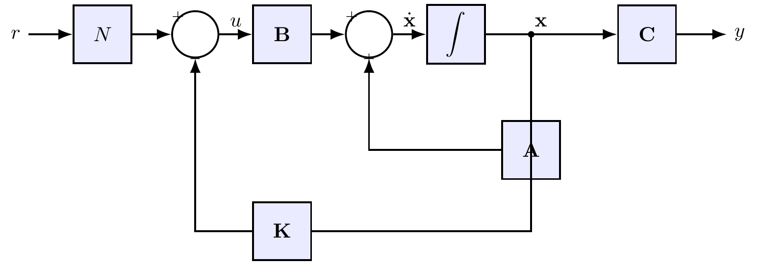
Realimentação de estados com ganho de referência N
Lei de controle u=Nr-Kx aplicada à planta em espaço de estados, com realimentação de todos os estados.
Ver código TikZ
% ---------------------------------------------------------------
% Realimentação de estados:  u = N r - K x ,  planta x_dot = A x + B u
% Bibliotecas (chunk .qmd): arrows.meta, positioning, calc
% ---------------------------------------------------------------
\begin{tikzpicture}[>=Latex, line width=0.9pt,
  block/.style={draw, minimum width=1.0cm, minimum height=1.0cm, fill=blue!8},
  sum/.style={draw, circle, minimum size=8mm, inner sep=0pt}]

  \node (r)          at (-1.5,0) {$r$};
  \node[block] (N)   at (0,0)    {$N$};
  \node[sum]   (si)  at (1.6,0)  {};
  \node[block] (B)   at (3.1,0)  {$\mathbf{B}$};
  \node[sum]   (ss)  at (4.6,0)  {};
  \node[block] (int) at (6.1,0)  {$\displaystyle\int$};
  \node[block] (C)   at (9.4,0)  {$\mathbf{C}$};
  \node (y)          at (11.0,0) {$y$};

  \node[block] (A)   at (7.4,-2.0) {$\mathbf{A}$};
  \node[block] (K)   at (3.1,-3.4) {$\mathbf{K}$};

  \coordinate (x) at (7.4,0);

  % sinais
  \node[font=\scriptsize] at ($(si)+(-0.30,0.30)$) {$+$};
  \node[font=\scriptsize] at ($(si)+(0,-0.42)$)    {$-$};
  \node[font=\scriptsize] at ($(ss)+(-0.30,0.30)$) {$+$};
  \node[font=\scriptsize] at ($(ss)+(0,-0.42)$)    {$+$};

  % cadeia direta
  \draw[->] (r) -- (N);
  \draw[->] (N) -- (si);
  \draw[->] (si) -- (B) node[midway, above] {$u$};
  \draw[->] (B) -- (ss);
  \draw[->] (ss) -- (int) node[midway, above] {$\dot{\mathbf{x}}$};
  \draw[->] (int) -- (C) node[pos=0.42, above] {$\mathbf{x}$};
  \draw[->] (C) -- (y);

  % realimentação A (+)
  \fill (x) circle (1.6pt);
  \draw[-]  (x) -- (A.north);
  \draw[->] (A.west) -| (ss);

  % realimentação de estados -K
  \draw[-]  (7.4,0) -- (7.4,-3.4) -- (K.east);
  \draw[->] (K.west) -| (si);

\end{tikzpicture}
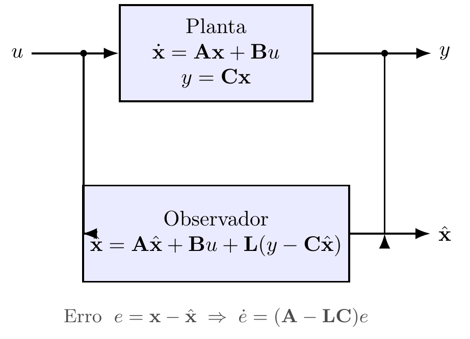
Observador de Luenberger
Diagrama de blocos do observador de Luenberger estimando o estado x a partir da entrada u e da saída y da planta.
Ver código TikZ
% ---------------------------------------------------------------
% Observador de Luenberger (nível de blocos)
%   Planta:     x_dot = A x + B u ,  y = C x
%   Observador: xhat_dot = A xhat + B u + L (y - C xhat)
% Bibliotecas (chunk .qmd): arrows.meta, positioning, calc
% ---------------------------------------------------------------
\begin{tikzpicture}[>=Latex, line width=0.9pt,
  big/.style={draw, minimum width=3.2cm, minimum height=1.6cm, fill=blue!8, align=center},
  sum/.style={draw, circle, minimum size=8mm, inner sep=0pt}]

  \node (u)             at (-1.5,0) {$u$};
  \node[big] (plant)    at (1.8,0)  {Planta\\$\dot{\mathbf{x}}=\mathbf{A}\mathbf{x}+\mathbf{B}u$\\$y=\mathbf{C}\mathbf{x}$};
  \node (y)             at (5.6,0)  {$y$};

  \node[big] (obs)      at (1.8,-3.0) {Observador\\$\dot{\hat{\mathbf{x}}}=\mathbf{A}\hat{\mathbf{x}}+\mathbf{B}u+\mathbf{L}(y-\mathbf{C}\hat{\mathbf{x}})$};
  \node (xhat)          at (5.6,-3.0) {$\hat{\mathbf{x}}$};

  % u para planta e observador
  \fill (-0.4,0) circle (1.6pt);
  \draw[->] (u) -- (plant);
  \draw[-]  (-0.4,0) -- (-0.4,-3.0);
  \draw[->] (-0.4,-3.0) -- (obs);

  % saída da planta
  \draw[->] (plant) -- (y);

  % y realimentado ao observador
  \fill (4.6,0) circle (1.6pt);
  \draw[-]  (4.6,0) -- (4.6,-1.6);
  \draw[->] (4.6,-1.6) -- (4.6,-3.0) -- (obs.east -| 4.6,-3.0);

  % estado estimado
  \draw[->] (obs) -- (xhat);

  \node[font=\small, gray!60!black] at (1.8,-4.4)
        {Erro $\;e=\mathbf{x}-\hat{\mathbf{x}}\;\Rightarrow\; \dot{e}=(\mathbf{A}-\mathbf{L}\mathbf{C})e$};

\end{tikzpicture}
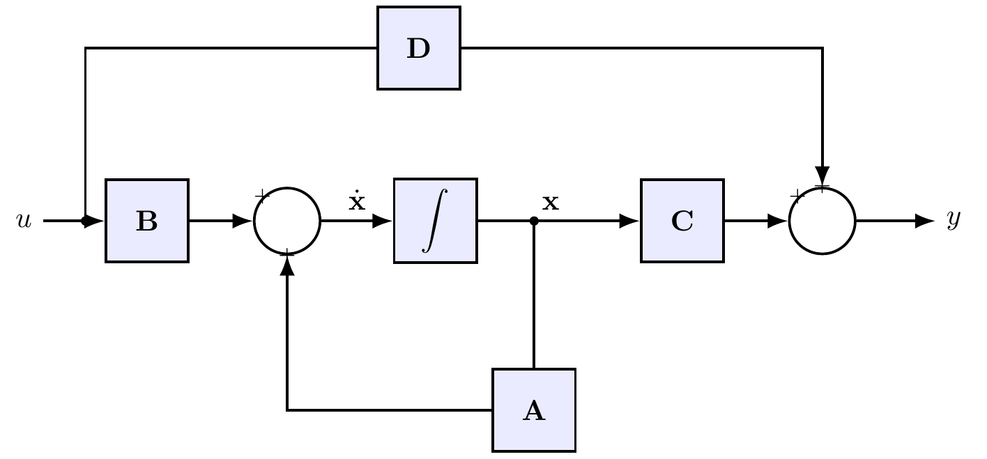
Diagrama de blocos em espaço de estados (malha aberta, com D)
Variante do diagrama em espaço de estados incluindo a matriz de transmissão direta D, além de A, B e C.
Ver código TikZ
% ---------------------------------------------------------------
% Diagrama de blocos do modelo de estados (malha aberta)
%   x_dot = A x + B u ,  y = C x + D u
% Bibliotecas (carregadas no chunk .qmd): arrows.meta, positioning, calc
% ---------------------------------------------------------------
\begin{tikzpicture}[>=Latex, line width=0.9pt,
  block/.style={draw, minimum width=1.0cm, minimum height=1.0cm, fill=blue!8},
  sum/.style={draw, circle, minimum size=8mm, inner sep=0pt}]

  % --- Cadeia direta ---
  \node (u)            at (0,0)    {$u$};
  \node[block] (B)     at (1.5,0)  {$\mathbf{B}$};
  \node[sum]   (s1)    at (3.2,0)  {};
  \node[block] (int)   at (5.0,0)  {$\displaystyle\int$};
  \node[block] (C)     at (8.0,0)  {$\mathbf{C}$};
  \node[sum]   (s2)    at (9.7,0)  {};
  \node (y)            at (11.3,0) {$y$};
  \node[block] (A)     at (6.2,-2.3) {$\mathbf{A}$};
  \node[block] (D)     at (4.8,2.1)  {$\mathbf{D}$};

  % Ponto de derivação do estado x
  \coordinate (x) at (6.2,0);

  % --- Sinais nos somadores ---
  \node[font=\scriptsize] at ($(s1)+(-0.30,0.30)$) {$+$};
  \node[font=\scriptsize] at ($(s1)+(0,-0.42)$)    {$+$};
  \node[font=\scriptsize] at ($(s2)+(-0.30,0.30)$) {$+$};
  \node[font=\scriptsize] at ($(s2)+(0,0.42)$)     {$+$};

  % --- Ligações cadeia direta ---
  \draw[->] (u) -- (B);
  \draw[->] (B) -- (s1);
  \draw[->] (s1) -- (int) node[midway, above] {$\dot{\mathbf{x}}$};
  \draw[->] (int) -- (C) node[pos=0.45, above] {$\mathbf{x}$};
  \draw[->] (C) -- (s2);
  \draw[->] (s2) -- (y);

  % --- Realimentação A (positiva: +Ax) ---
  \fill (x) circle (1.6pt);
  \draw[-]  (x) -- (A.north);
  \draw[->] (A.west) -| (s1);

  % --- Transmissão direta D ---
  \fill (0.75,0) circle (1.6pt);
  \draw[-]  (0.75,0) |- (D.west);
  \draw[->] (D.east) -| (s2);

\end{tikzpicture}
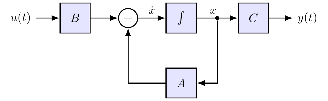
Diagrama de blocos em espaço de estados (malha aberta)
Representação em diagrama de blocos do modelo em espaço de estados x_dot=Ax+Bu, y=Cx, em malha aberta.
Ver código TikZ
\tikzset{
    % Estilos dos blocos
    block/.style = {draw, fill=blue!10, rectangle, minimum height=2.5em, minimum width=2.5em, line width=0.8pt},
    % Somador 30% menor (reduzido de 1pt/Large para algo mais compacto)
    sum/.style = {draw, fill=white, circle, inner sep=2pt, line width=0.8pt},
    dot/.style = {fill, circle, inner sep=1.2pt}
}

\begin{tikzpicture}[auto, node distance=1.2cm, >=Latex, line width=0.8pt]
    % Ajuste global da escala da ponta da seta para ser proporcional ao diagrama menor
    \begin{scope}[arrows={-Latex[scale=0.8]}]

        % Nós (Posicionamento com distâncias reduzidas)
        \node (input) at (0,0) {};
        \node [block, right=0.7cm of input] (matrixB) {$B$};
        \node [sum, right=0.8cm of matrixB] (sum) {$+$};
        \node [block, right=0.8cm of sum] (int) {$\int$};
        \node [block, right=1.2cm of int] (matrixC) {$C$};
        \node (output) [right=0.7cm of matrixC] {};

        % Bloco de realimentação
        \node [block, below=1cm of int] (matrixA) {$A$};

        % Caminho Principal
        \draw [->] (input) -- (matrixB) node[left, pos=0] {$u(t)$};
        \draw [->] (matrixB) -- (sum);
        \draw [->] (sum) -- node[above, font=\small] {$\dot{x}$} (int);
        \draw [->] (int) -- (matrixC) node[above, pos=0.4, font=\small] {$x$};
        \draw [->] (matrixC) -- (output) node[right, pos=1] {$y(t)$};

        % Ponto de derivação e Realimentação
        \node [dot] (point) at ($(int.east)!0.5!(matrixC.west)$) {};
        \draw [->] (point) |- (matrixA);
        \draw [->] (matrixA) -| (sum);

    \end{scope}
\end{tikzpicture}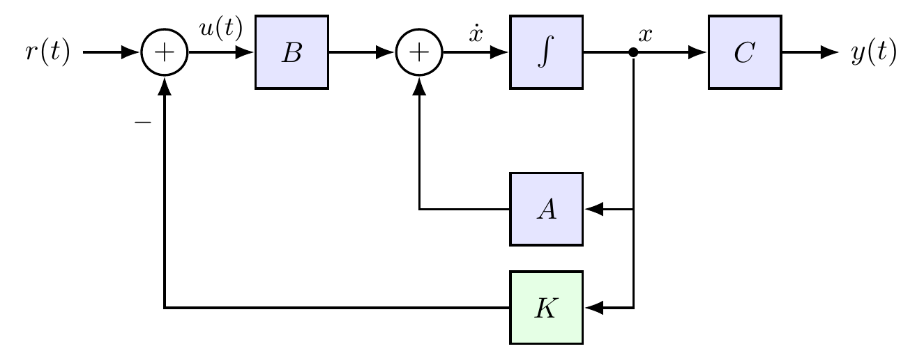
Diagrama de blocos em espaço de estados (malha fechada)
Realimentação de estados u=r-Kx sobre o modelo em espaço de estados, incluindo a matriz de ganho K.
Ver código TikZ
\tikzset{
    block/.style = {draw, fill=blue!10, rectangle, minimum height=2.5em, minimum width=2.5em, line width=0.8pt},
    sum/.style   = {draw, fill=white, circle, inner sep=2pt, line width=0.8pt},
    dot/.style   = {fill, circle, inner sep=1.2pt}
}
\begin{tikzpicture}[auto, node distance=1.2cm, >=Latex, line width=0.8pt]
    \begin{scope}[arrows={-Latex[scale=0.8]}]

        % --- Malha Direta ---
        \node (input) at (0,0) {};
        \node [sum,   right=0.7cm of input]   (sumU)    {$+$};
        \node [block, right=0.8cm of sumU]    (matrixB) {$B$};
        \node [sum,   right=0.8cm of matrixB] (sumX)    {$+$};
        \node [block, right=0.8cm of sumX]    (int)     {$\int$};
        \node [block, right=1.5cm of int]     (matrixC) {$C$};
        \node (output) [right=0.7cm of matrixC] {};

        % --- Malhas de Realimentação ---
        \node [block,                  below=1.0cm of int] (matrixA) {$A$};
        \node [block, fill=green!10,   below=2.2cm of int] (matrixK) {$K$};

        % --- Conexões ---

        % Referência r(t)
        \draw [->] (input) -- (sumU) node[left, pos=0] {$r(t)$};

        % u(t)
        \draw [->] (sumU)    -- node[above, font=\small] {$u(t)$} (matrixB);
        \draw [->] (matrixB) -- (sumX);

        % Dinâmica de estados
        \draw [->] (sumX) -- node[above, font=\small] {$\dot{x}$} (int);
        \draw [->] (int)  -- (matrixC) node[above, pos=0.5, font=\small] {$x$};
        \draw [->] (matrixC) -- (output) node[right, pos=1] {$y(t)$};

        % Ponto de derivação do estado x
        \node [dot] (pointX) at ($(int.east)!0.4!(matrixC.west)$) {};

        % Realimentação interna (A)
        \draw [->] (pointX) |- (matrixA);
        \draw [->] (matrixA) -| (sumX);

        % Realimentação de controle (K)
        \draw [->] (pointX) |- (matrixK);
        \draw [->] (matrixK) -| node[left, pos=0.9, font=\small] {$-$} (sumU);

    \end{scope}
\end{tikzpicture}
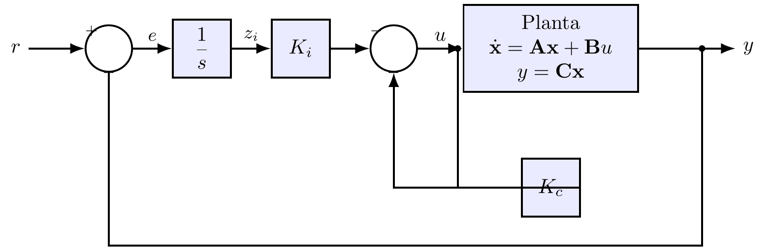
Servomecanismo com ação integral
Controle servo com ação integral do erro (estado z_i) somada à realimentação de estados -Kc x.
Ver código TikZ
% ---------------------------------------------------------------
% Servomecanismo (ação integral):  zi_dot = r - y ,  u = -Kc x - Ki zi
% Bibliotecas (chunk .qmd): arrows.meta, positioning, calc
% ---------------------------------------------------------------
\begin{tikzpicture}[>=Latex, line width=0.9pt,
  block/.style={draw, minimum width=1.0cm, minimum height=1.0cm, fill=blue!8},
  big/.style={draw, minimum width=3.0cm, minimum height=1.5cm, fill=blue!8, align=center},
  sum/.style={draw, circle, minimum size=8mm, inner sep=0pt}]

  \node (r)            at (-1.6,0) {$r$};
  \node[sum]   (se)    at (0,0)    {};
  \node[block] (intz)  at (1.6,0)  {$\displaystyle\frac{1}{s}$};
  \node[block] (Ki)    at (3.3,0)  {$K_i$};
  \node[sum]   (su)    at (4.9,0)  {};
  \node[big]   (plant) at (7.6,0)  {Planta\\$\dot{\mathbf{x}}=\mathbf{A}\mathbf{x}+\mathbf{B}u$\\$y=\mathbf{C}\mathbf{x}$};
  \node (y)            at (11.0,0) {$y$};

  \node[block] (Kc)    at (7.6,-2.4) {$K_c$};

  % sinais
  \node[font=\scriptsize] at ($(se)+(-0.30,0.30)$) {$+$};
  \node[font=\scriptsize] at ($(se)+(0,-0.42)$)    {$-$};
  \node[font=\scriptsize] at ($(su)+(-0.30,0.30)$) {$-$};
  \node[font=\scriptsize] at ($(su)+(0,-0.42)$)    {$-$};

  % cadeia direta
  \draw[->] (r) -- (se);
  \draw[->] (se) -- (intz) node[midway, above, font=\small] {$e$};
  \draw[->] (intz) -- (Ki) node[midway, above, font=\small] {$z_i$};
  \draw[->] (Ki) -- (su);
  \draw[->] (su) -- (plant) node[midway, above] {$u$};
  \draw[->] (plant) -- (y);

  % realimentação de y ao erro
  \fill (10.2,0) circle (1.6pt);
  \draw[-]  (10.2,0) -- (10.2,-3.4) -- (0,-3.4) -- (se);

  % realimentação de estados -Kc
  \fill (6.0,0) circle (1.6pt);
  \draw[-]  (6.0,0) -- (6.0,-2.4) -- (Kc.east);
  \draw[->] (Kc.west) -| (su);

\end{tikzpicture}
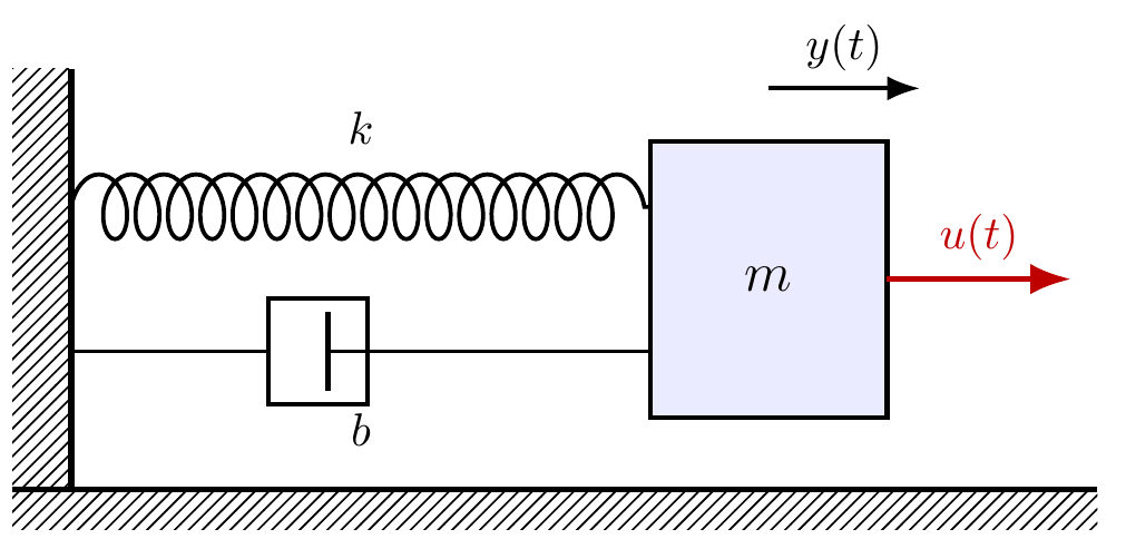
Sistema massa-mola-amortecedor (variante)
Outra representação gráfica do sistema massa-mola-amortecedor, com força de entrada u(t) e saída y(t).
Ver código TikZ
% ---------------------------------------------------------------
% Sistema massa-mola-amortecedor
% Bibliotecas (carregadas no chunk .qmd):
%   arrows.meta, positioning, calc, decorations.pathmorphing, patterns
% ---------------------------------------------------------------
\begin{tikzpicture}[>=Latex, line width=0.9pt]

  % --- Parede fixa ---
  \fill[pattern=north east lines] (-0.45,-1.6) rectangle (0,1.6);
  \draw[line width=1.3pt] (0,-1.6) -- (0,1.6);

  % --- Massa ---
  \def\mx{4.4}
  \draw[fill=blue!8, line width=1pt] (\mx,-1.05) rectangle (\mx+1.8,1.05);
  \node at (\mx+0.9,0) {\large $m$};

  % --- Mola (ramo superior) ---
  \draw[decorate, decoration={coil, aspect=0.6, segment length=7pt, amplitude=7pt}]
        (0,0.55) -- (\mx,0.55);
  \node at (\mx/2,1.15) {$k$};

  % --- Amortecedor (ramo inferior) ---
  \draw (0,-0.55) -- (1.5,-0.55);
  \draw (1.5,-0.95) rectangle (2.25,-0.15);
  \draw[line width=1.1pt] (1.95,-0.85) -- (1.95,-0.25);
  \draw (1.95,-0.55) -- (\mx,-0.55);
  \node at (\mx/2,-1.15) {$b$};

  % --- Força de entrada ---
  \draw[->, red!75!black, line width=1.3pt]
        (\mx+1.8,0) -- (\mx+3.2,0) node[midway, above] {$u(t)$};

  % --- Deslocamento ---
  \draw[->] (\mx+0.9,1.45) -- (\mx+2.05,1.45) node[midway, above] {$y(t)$};

  % --- Solo ---
  \fill[pattern=north east lines] (-0.45,-1.9) rectangle (\mx+3.4,-1.6);
  \draw[line width=1.3pt] (-0.45,-1.6) -- (\mx+3.4,-1.6);

\end{tikzpicture}
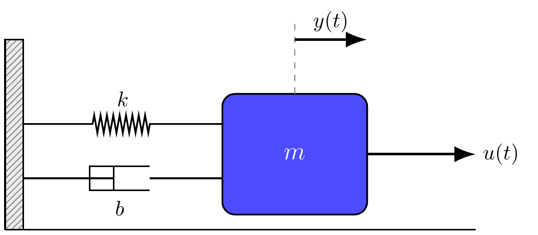
Sistema massa-mola-amortecedor
Sistema massa-mola-amortecedor com entrada de força u(t) e saída de deslocamento y(t), usado na modelagem em espaço de estados.
Ver código TikZ
\begin{tikzpicture}[every node/.style={outer sep=0pt, thick}]
\tikzset{
    preenchimento/.style={fill=lightgray!30},
    hachura/.style={pattern=north east lines, pattern color=gray},
    mola/.style={decorate, decoration={zigzag, segment length=3pt, amplitude=4.2pt, pre length=1.15cm, post length=1.15cm}, draw=black, thick},
    massa/.style={draw, fill=blue!70!white, text=white, font=\large\bfseries, rounded corners=6pt}
}
\node[preenchimento, minimum width=0.3cm, minimum height=3.15cm, anchor=south east] (parede_fundo) at (0,-0.16) {};
\node[hachura, minimum width=0.3cm, minimum height=3.15cm, anchor=south east] (parede_listras) at (0,-0.16) {};
\draw[thick] (-0.3, -0.15) -- (7.5, -0.15);
\draw[thick] (-0.3, -0.15) -- (-0.3, 3) -- (0, 3) -- (0,-0.15);
\node[massa, minimum width=2.4cm, minimum height=2.0cm, anchor=south] (M) at (4.5, 0.1) {$m$};
\draw[mola] (0, 1.6) -- (M.west |- 0, 1.6) node[midway, above=5pt] {$k$};
\begin{scope}[yshift=0.7cm]
    \draw[thick] (0,0) -- (1.5,0);
    \draw[thick] (1.5,-0.2) -- (1.5,0.2);
    \draw[thick] (2.1,0.2) -- (1.1,0.2) -- (1.1,-0.2) -- (2.1,-0.2);
    \draw[thick] (2.1,0) -- (M.west |- 0, 0);
    \node at (1.6, -0.5) {$b$};
\end{scope}
\draw[-{Latex[scale=1.2]}, very thick, black] (M.east) -- ++(1.8,0) node[right] {$u(t)$};
\draw[dashed, gray] (M.center |- 0, 2.1) -- ++(0, 1.2);
\draw[-{Latex[scale=1.2]}, very thick, black] ($(M.center |- 0, 3.0)$) -- ++(1.2,0) node[midway, above] {$y(t)$};
\end{tikzpicture}
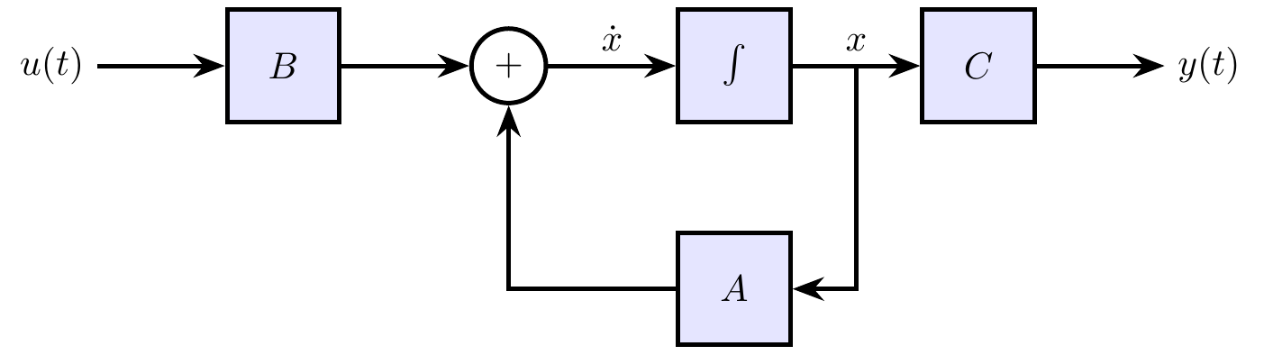
Diagrama de Blocos do Modelo em Espaço de Estados
Representação canônica ẋ = Ax + Bu, y = Cx em diagrama de blocos, com integrador e realimentação interna pela matriz A.
Ver código TikZ
\begin{tikzpicture}[
    bloco/.style={
        draw,
        rectangle,
        minimum height=3em,
        minimum width=3em,
        fill=blue!10,
        line width=1.2pt
    },
    somador/.style={
        draw,
        circle,
        minimum size=7mm,
        line width=1.2pt
    },
    vetor/.style={
        ->,
        >=Stealth,
        line width=1.2pt
    },
    % Distâncias reduzidas para compactar o diagrama
    node distance=1.0cm and 1.2cm
]

    % Nós
    \node (input) {$u(t)$};
    \node [bloco, right=of input] (B) {$B$};
    \node [somador, right=of B] (sum) {$+$};
    \node [bloco, right=of sum] (int) {$\int$};
    \node [bloco, right=of int] (C) {$C$};
    \node [right=of C] (output) {$y(t)$};
    \node [bloco, below=of int] (A) {$A$};

    % Conexões
    \draw [vetor] (input) -- (B);
    \draw [vetor] (B) -- (sum);
    \draw [vetor] (sum) -- node[above] {$\dot{x}$} (int);
    \draw [vetor] (int) -- node[above, name=x] {$x$} (C);
    \draw [vetor] (C) -- (output);

    % Realimentação
    \draw [vetor] (x) |- (A);
    \draw [vetor] (A) -| (sum);

\end{tikzpicture}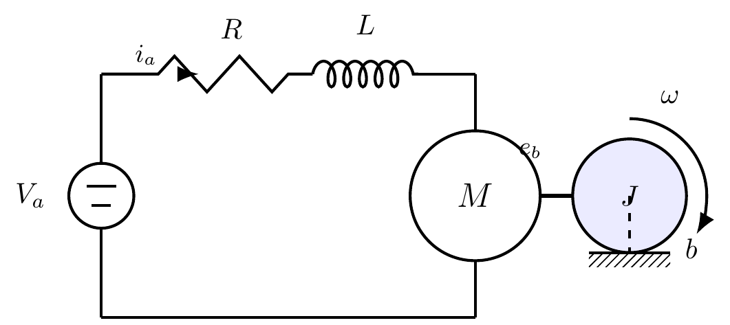
Motor CC: circuito de armadura e carga mecânica
Motor CC com resistência e indutância de armadura, força contra-eletromotriz e carga mecânica com inércia J e atrito b.
Ver código TikZ
% ---------------------------------------------------------------
% Motor CC: circuito de armadura (Va, R, L, eb) + carga mecânica (J, b)
%   Va = L dia/dt + R ia + eb ,  eb = Ke·w
%   J dw/dt = T - b·w ,  T = Kt·ia
% Bibliotecas (carregadas no chunk .qmd):
%   arrows.meta, positioning, calc, decorations.pathmorphing
% ---------------------------------------------------------------
\begin{tikzpicture}[>=Latex, line width=1pt]

  % --- Fonte de armadura Va ---
  \draw (0,0) -- (0,1.1);
  \draw (0,1.9) -- (0,3);
  \draw (0,1.5) circle (0.4);
  \draw (-0.18,1.62) -- (0.18,1.62);
  \draw (-0.12,1.38) -- (0.12,1.38);
  \node[left] at (-0.55,1.5) {$V_a$};

  % --- Resistor R ---
  \draw (0,3) -- (0.7,3)
        -- (0.9,3.22) -- (1.3,2.78) -- (1.7,3.22) -- (2.1,2.78) -- (2.3,3) -- (2.6,3);
  \node[above] at (1.6,3.3) {$R$};

  % --- Indutor L ---
  \draw[decorate, decoration={coil, aspect=0.55, segment length=5.5pt, amplitude=4.5pt}]
        (2.6,3) -- (3.9,3);
  \node[above] at (3.25,3.35) {$L$};
  \draw (3.9,3) -- (4.6,3);

  % --- Corrente de armadura ia ---
  \draw[->] (0.95,3) -- (1.2,3);
  \node[above, font=\small] at (0.55,2.98) {$i_a$};

  % --- Motor (força contra-eletromotriz eb) ---
  \draw (4.6,3) -- (4.6,2.3);
  \draw (4.6,1.5) circle (0.8);
  \node at (4.6,1.5) {\large $M$};
  \draw (4.6,0.7) -- (4.6,0);
  \node[right, font=\small] at (5.0,2.05) {$e_b$};

  % --- Retorno ---
  \draw (0,0) -- (4.6,0);

  % --- Eixo / acoplamento mecânico ---
  \draw[line width=1.4pt] (5.4,1.5) -- (6.5,1.5);

  % --- Inércia J (disco) ---
  \draw[fill=blue!8] (6.5,1.5) circle (0.7);
  \node at (6.5,1.5) {$J$};
  % velocidade angular w
  \draw[->, line width=1pt] (6.5,2.45) arc (90:-30:0.95);
  \node[above] at (7.0,2.5) {$\omega$};
  % atrito viscoso b (apoio)
  \draw (6.0,0.8) -- (7.0,0.8);
  \fill[pattern=north east lines] (6.0,0.62) rectangle (7.0,0.8);
  \draw[dashed] (6.5,1.5) -- (6.5,0.8);
  \node[right] at (7.05,0.85) {$b$};

\end{tikzpicture}
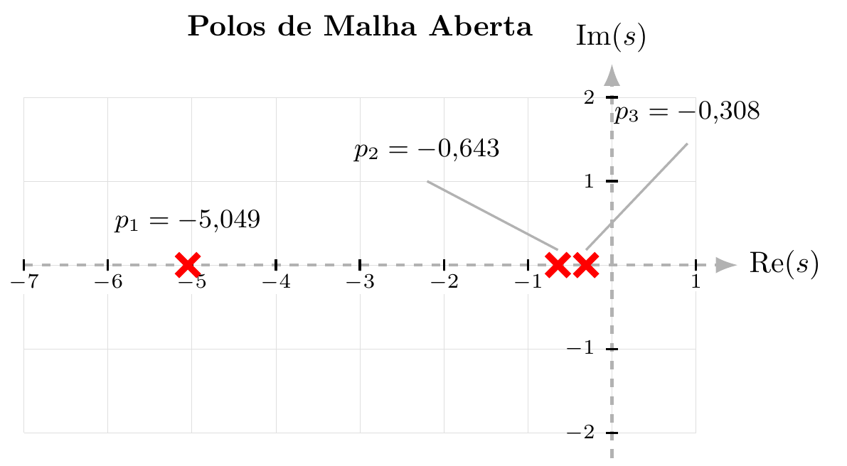
Mapa de polos no plano-s
Polos de malha aberta representados no plano complexo s, com valores numéricos indicados.
Ver código TikZ
% ---------------------------------------------------------------
% Mapa de polos no plano-s  (recriação de "Polos de Malha Aberta")
% Bibliotecas (carregadas no chunk .qmd): arrows.meta
% ---------------------------------------------------------------
\begin{tikzpicture}[>=Latex, line width=0.8pt]

  % --- Grade ---
  \draw[help lines, gray!25] (-7,-2) grid[step=1] (1,2);

  % --- Eixos ---
  \draw[->, gray!60, dashed, line width=1pt] (-7,0) -- (1.5,0)
        node[right, black] {$\mathrm{Re}(s)$};
  \draw[->, gray!60, dashed, line width=1pt] (0,-2.3) -- (0,2.4)
        node[above, black] {$\mathrm{Im}(s)$};

  % --- Marcações ---
  \foreach \x in {-7,-6,-5,-4,-3,-2,-1,1}
    \draw (\x,0.07)--(\x,-0.07) node[below, font=\scriptsize, fill=white, inner sep=1pt]{$\x$};
  \foreach \y in {-2,-1,1,2}
    \draw (0.07,\y)--(-0.07,\y) node[left, font=\scriptsize]{$\y$};

  % --- Polos (x vermelho) ---
  \def\polo(#1,#2){%
    \draw[red, line width=2.2pt] (#1-0.13,#2-0.13)--(#1+0.13,#2+0.13);
    \draw[red, line width=2.2pt] (#1-0.13,#2+0.13)--(#1+0.13,#2-0.13);}
  \polo(-5.049,0)
  \polo(-0.643,0)
  \polo(-0.308,0)

  % --- Rótulos sem sobreposição ---
  \node[above, font=\small] at (-5.049,0.25) {$p_1=-5{,}049$};

  \node[above, font=\small] at (-2.2,1.1) {$p_2=-0{,}643$};
  \draw[gray!60] (-2.2,1.0) -- (-0.643,0.18);

  \node[above, font=\small] at (0.9,1.55) {$p_3=-0{,}308$};
  \draw[gray!60] (0.9,1.45) -- (-0.308,0.18);

  % --- Título ---
  \node[font=\bfseries] at (-3,2.85) {Polos de Malha Aberta};

\end{tikzpicture}