Métodos Numéricos
6 figura(s) nesta categoria. Fonte em figuras/metodos-numericos/.
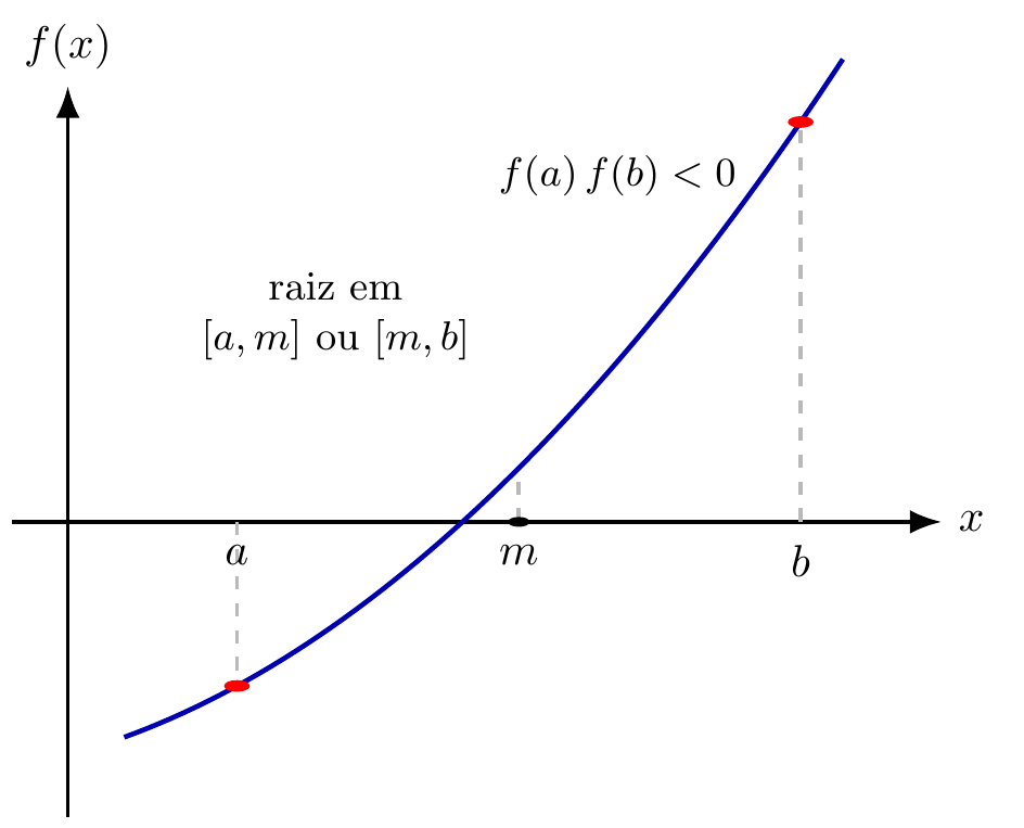
Método da bisseção
Iteração do método da bisseção: f(a)f(b)<0 garante uma raiz no intervalo, refinado pelo ponto médio m.
Ver código TikZ
% Método da bisseção: f(a)f(b)<0, ponto médio m
% Bibliotecas (chunk .qmd): arrows.meta
\begin{tikzpicture}[>=Latex, xscale=2.2, yscale=1.0, line width=0.9pt]
  \draw[->] (0.4,0) -- (3.7,0) node[right] {$x$};
  \draw[->] (0.6,-2.3) -- (0.6,3.4) node[above] {$f(x)$};

  % f(x) = 0.5 x^2 - 2  (raiz em x = 2)
  \draw[blue!70!black, line width=1.1pt]
        plot[domain=0.8:3.35, samples=60] (\x, {0.5*\x*\x - 2});

  \def\a{1.2}\def\b{3.2}\def\m{2.2}
  \foreach \p/\lab in {\a/a, \b/b, \m/m}{
    \draw[dashed, gray!55] (\p,0) -- (\p, {0.5*\p*\p - 2});
    \node[below] at (\p,-0.05) {$\lab$};
  }
  \fill[red] (\a, {0.5*\a*\a - 2}) circle (1.3pt);
  \fill[red] (\b, {0.5*\b*\b - 2}) circle (1.3pt);
  \fill (\m,0) circle (1.1pt);
  \node[font=\small] at (2.55,2.7) {$f(a)\,f(b) < 0$};
  \node[font=\small, align=center] at (1.55,1.6) {raiz em\\$[a,m]$ ou $[m,b]$};
\end{tikzpicture}
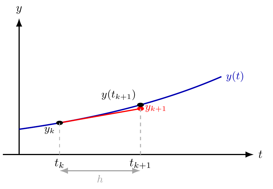
Passo do método de Euler
Avanço de um passo pelo método de Euler usando a reta tangente, comparado com a solução exata da EDO.
Ver código TikZ
% Passo de Euler: avanço pela tangente; comparação com a solução exata
% Bibliotecas (chunk .qmd): arrows.meta
\begin{tikzpicture}[>=Latex, xscale=2.4, yscale=1.5, line width=0.9pt]
  \draw[->] (0.3,0) -- (3.4,0) node[right] {$t$};
  \draw[->] (0.5,0) -- (0.5,2.7) node[above] {$y$};

  % solução exata y = 0.4 e^{0.45 t}
  \draw[blue!70!black, line width=1.1pt]
        plot[domain=0.5:3.0, samples=60] (\x, {0.4*exp(0.45*\x)})
        node[right, font=\small] {$y(t)$};

  \def\tk{1.0}\def\tn{2.0}
  \pgfmathsetmacro\yk{0.4*exp(0.45*\tk)}
  \pgfmathsetmacro\slope{0.45*\yk}
  \pgfmathsetmacro\yeuler{\yk + \slope*(\tn-\tk)}

  % passo de Euler (tangente)
  \draw[red, line width=1pt] (\tk,\yk) -- (\tn,\yeuler);
  \fill (\tk,\yk) circle (1.2pt);
  \fill[red] (\tn,\yeuler) circle (1.2pt) node[right, font=\small] {$y_{k+1}$};
  \fill (\tn, {0.4*exp(0.45*\tn)}) circle (1.2pt) node[above left, font=\small] {$y(t_{k+1})$};

  \draw[dashed, gray!55] (\tk,0) -- (\tk,\yk);
  \draw[dashed, gray!55] (\tn,0) -- (\tn,\yeuler);
  \node[below] at (\tk,0) {$t_k$};
  \node[below] at (\tn,0) {$t_{k+1}$};
  \node[below left, font=\small] at (\tk,\yk) {$y_k$};
  \draw[<->, gray!70] (\tk,-0.32) -- (\tn,-0.32) node[midway, below, font=\small] {$h$};
\end{tikzpicture}
Método de Newton
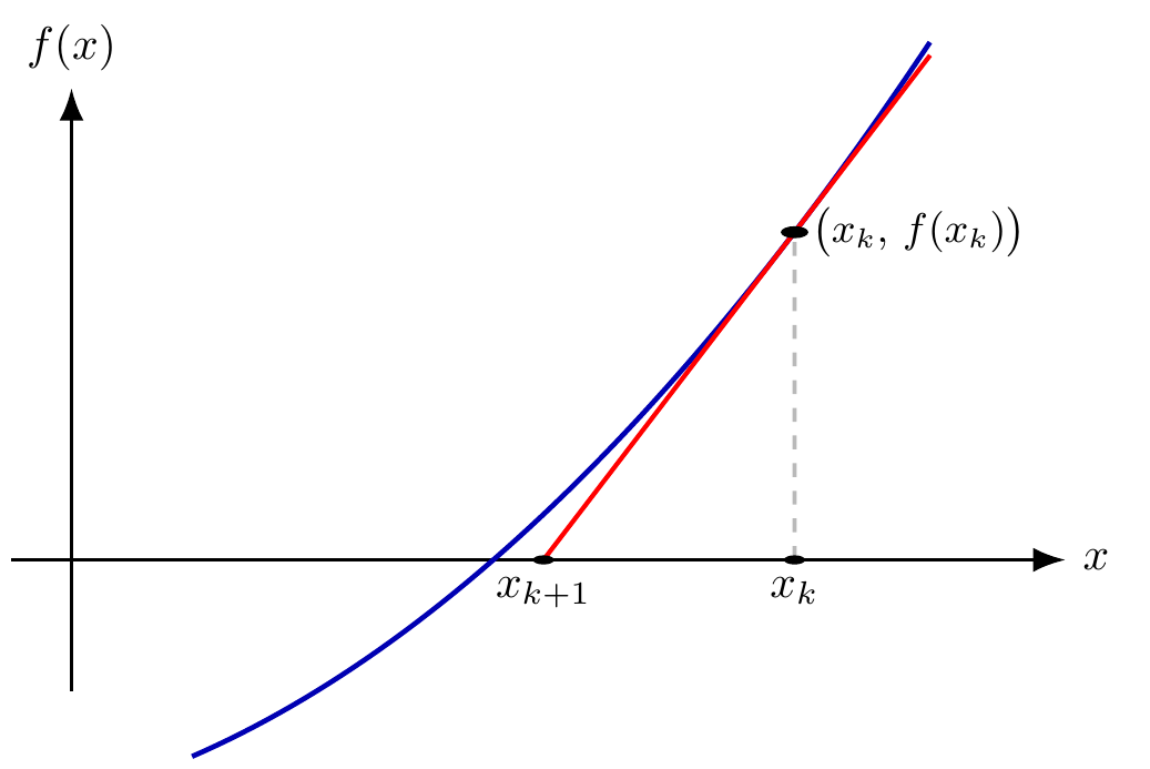
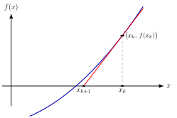
Iteração geométrica do método de Newton: a reta tangente em x_k cruza o eixo x em x_{k+1}.
Ver código TikZ
% Método de Newton: reta tangente em x_k cruza o eixo em x_{k+1}
% Bibliotecas (chunk .qmd): arrows.meta
\begin{tikzpicture}[>=Latex, xscale=2.3, yscale=1.0, line width=0.9pt]
  \draw[->] (0.4,0) -- (3.9,0) node[right] {$x$};
  \draw[->] (0.6,-1.0) -- (0.6,3.6) node[above] {$f(x)$};

  % f(x) = 0.5 x^2 - 2
  \draw[blue!70!black, line width=1.1pt]
        plot[domain=1.0:3.45, samples=60] (\x, {0.5*\x*\x - 2});

  \def\xk{3.0}\def\xn{2.1667}      % x_{k+1} = x_k - f/f'
  \coordinate (P) at (\xk, {0.5*\xk*\xk - 2});
  % tangente (inclinação f'(x_k)=x_k=3)
  \draw[red, line width=1pt] (\xn,0) -- (P);
  \draw[red, line width=1pt] (P) -- (3.45, {0.5*\xk*\xk - 2 + 3*(3.45-\xk)});

  \draw[dashed, gray!55] (\xk,0) -- (P);
  \fill (P) circle (1.3pt);
  \fill (\xk,0) circle (1pt) node[below] {$x_k$};
  \fill (\xn,0) circle (1pt) node[below] {$x_{k+1}$};
  \node[right, font=\small] at (P) {$\bigl(x_k,\,f(x_k)\bigr)$};
\end{tikzpicture}
Iteração de ponto fixo (cobweb)
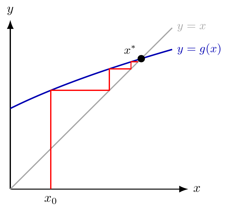
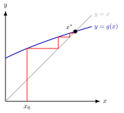
Iteração x=g(x) representada como diagrama de teia de aranha (cobweb), convergindo ao ponto fixo x*.
Ver código TikZ
% Iteração de ponto fixo x = g(x) com cobweb
% Bibliotecas (chunk .qmd): arrows.meta
\begin{tikzpicture}[>=Latex, scale=2.2, line width=0.9pt]
  \draw[->] (0,0) -- (2.2,0) node[right] {$x$};
  \draw[->] (0,0) -- (0,2.1) node[above] {$y$};

  % reta y = x
  \draw[gray!70] (0,0) -- (2.0,2.0) node[right, font=\small] {$y=x$};
  % g(x) = sqrt(x+1)
  \draw[blue!70!black, line width=1.1pt]
        plot[domain=0:2.0, samples=60] (\x, {sqrt(\x+1)})
        node[right, font=\small] {$y=g(x)$};

  % cobweb (valores pré-computados)
  \draw[red, line width=0.9pt]
        (0.5,0) -- (0.5,1.2247) -- (1.2247,1.2247)
        -- (1.2247,1.4914) -- (1.4914,1.4914)
        -- (1.4914,1.5785) -- (1.5785,1.5785);

  % ponto fixo
  \fill (1.618,1.618) circle (1.3pt);
  \node[above left, font=\small] at (1.618,1.618) {$x^{*}$};
  \node[below] at (0.5,-0.03) {$x_0$};
\end{tikzpicture}
Regra de Simpson
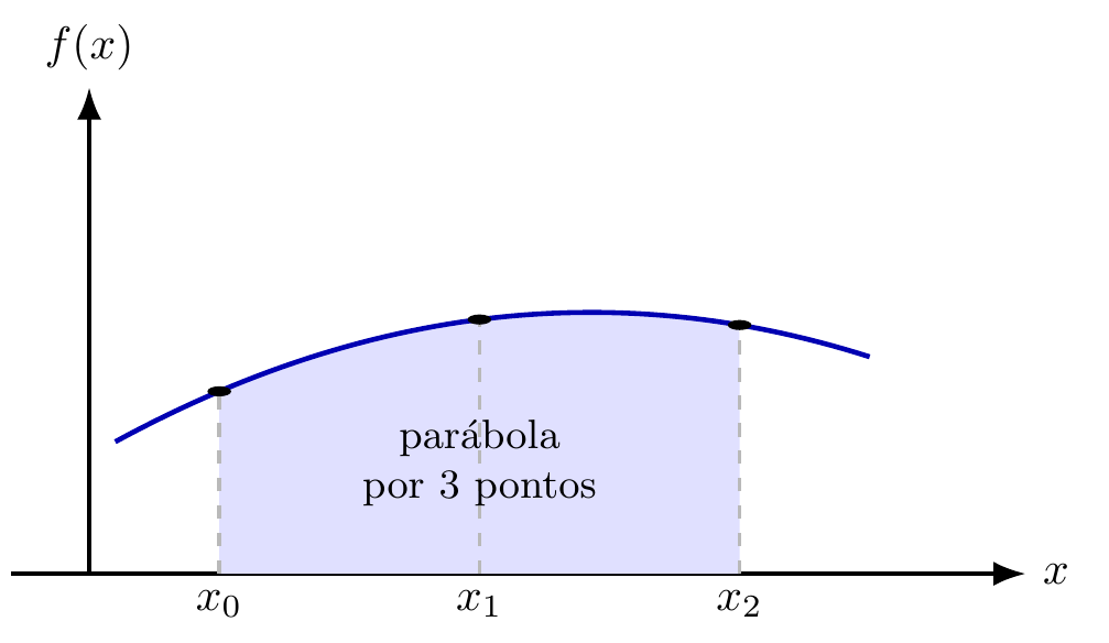
Aproximação da integral por uma parábola passando por três pontos (x0,x1,x2), base da regra de Simpson.
Ver código TikZ
% Regra de Simpson: parábola por 3 pontos (x0, x1, x2)
% Bibliotecas (chunk .qmd): arrows.meta
\begin{tikzpicture}[>=Latex, xscale=2.0, yscale=0.85, line width=0.9pt]
  \draw[->] (0.2,0) -- (4.1,0) node[right] {$x$};
  \draw[->] (0.5,0) -- (0.5,4.4) node[above] {$f(x)$};

  \def\xz{1.0}\def\xu{2.0}\def\xd{3.0}
  % f(x) = -0.35 x^2 + 1.7 x + 0.3  (parábola — coincide com a interpoladora)
  \fill[blue!12]
        plot[domain=\xz:\xd, samples=40] (\x, {-0.35*\x*\x + 1.7*\x + 0.3})
        -- (\xd,0) -- (\xz,0) -- cycle;
  \draw[blue!70!black, line width=1.1pt]
        plot[domain=0.6:3.5, samples=60] (\x, {-0.35*\x*\x + 1.7*\x + 0.3});

  \foreach \p/\lab in {\xz/{x_0}, \xu/{x_1}, \xd/{x_2}}{
    \draw[dashed, gray!55] (\p,0) -- (\p, {-0.35*\p*\p + 1.7*\p + 0.3});
    \fill (\p, {-0.35*\p*\p + 1.7*\p + 0.3}) circle (1.3pt);
    \node[below] at (\p,0) {$\lab$};
  }
  \node[font=\small, align=center] at (2.0,1.0) {parábola\\por 3 pontos};
\end{tikzpicture}
Regra do trapézio
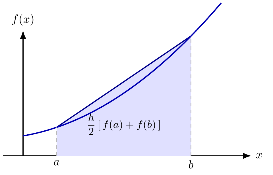
Aproximação da integral pela área do trapézio formado pela corda entre (a,f(a)) e (b,f(b)).
Ver código TikZ
% Regra do trapézio: corda entre (a,f(a)) e (b,f(b))
% Bibliotecas (chunk .qmd): arrows.meta
\begin{tikzpicture}[>=Latex, xscale=2.0, yscale=0.85, line width=0.9pt]
  \draw[->] (0.2,0) -- (3.9,0) node[right] {$x$};
  \draw[->] (0.5,0) -- (0.5,4.4) node[above] {$f(x)$};

  \def\a{1.0}\def\b{3.0}
  % área do trapézio
  \fill[blue!12] (\a,0) -- (\a,{0.4*\a*\a+0.6}) -- (\b,{0.4*\b*\b+0.6}) -- (\b,0) -- cycle;
  % corda
  \draw[blue!55!black, line width=1pt] (\a,{0.4*\a*\a+0.6}) -- (\b,{0.4*\b*\b+0.6});
  % curva f(x)=0.4x^2+0.6
  \draw[blue!70!black, line width=1.1pt]
        plot[domain=0.5:3.45, samples=60] (\x, {0.4*\x*\x+0.6});

  \draw[dashed, gray!55] (\a,0) -- (\a,{0.4*\a*\a+0.6});
  \draw[dashed, gray!55] (\b,0) -- (\b,{0.4*\b*\b+0.6});
  \node[below] at (\a,0) {$a$};
  \node[below] at (\b,0) {$b$};
  \node[font=\small] at (2.0,1.1) {$\dfrac{h}{2}\,[\,f(a)+f(b)\,]$};
\end{tikzpicture}