Eletronica Potencia
2 figura(s) nesta categoria. Fonte em figuras/eletronica-potencia/.
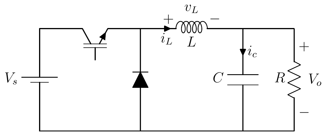
Conversor Buck
Topologia do conversor CC-CC Buck: chave IGBT, diodo de roda livre, indutor, capacitor e carga resistiva.
Ver código TikZ
\begin{circuitikz}[american]
    % --- CONFIGURAÇÕES LOCAIS (Substituem as opções de pacote) ---
    \ctikzset{
        inductor=cute,       % Equivalente a cuteinductors
        label/align=smart,   % Equivalente a smartlabels
        bipoles/thickness=0.7,
        bipoles/length=1.5cm,
        bipoles/resistor/width=0.7,
        bipoles/resistor/height=0.25,
        bipoles/diode/height=0.3,
        bipoles/diode/width=0.3,
        tripoles/thickness=0.5,
        bipoles/battery1/height=0.7
    }

    \tikzset{
        nodes={font=\large}, % Forma segura de definir fonte sem loop infinito
        every path/.style={line width=0.9pt, line cap=round, line join=round}
    }

    % --- DESENHO DO CIRCUITO ---
    \coordinate (VBottom) at (0,0);

    % Fonte de entrada
    \draw (VBottom) to [battery1, l=$V_{s}$, invert] ++(0,3) coordinate (VTop);

    % Chave IGBT
    \draw (VTop) to [short] ++(0.8,0)
        node [nigbt, anchor=C, rotate=90] (nigbt1){};

    % Conexões superiores (Diodo e Indutor)
    \draw (nigbt1.E) to [short] ++(0.5,0) coordinate (DiodeTop)
          to [short] ++(0.5,0)
          to [L, l_=$L$, v^=$v_L$, i>_=$i_L$] ++ (2,0) coordinate (InductorRight);

    % Diodo de roda livre
    \draw (DiodeTop) to [D*, invert] (DiodeTop|-VBottom);

    % Capacitor e Carga
    \draw (InductorRight) to [short] ++(0.5,0) coordinate (CapacitorTop)
          to [C, l_=$C$, i>^=$i_c$] (CapacitorTop|-VBottom);

    \draw (CapacitorTop) to [short] ++(1.5,0) coordinate (ResistorTop)
          to [R, l_=$R$, v^=$V_{o}$] (ResistorTop|-VBottom) coordinate (ResistorBottom);

    % Fechamento da malha inferior
    \draw (ResistorBottom) -- (VBottom);

\end{circuitikz}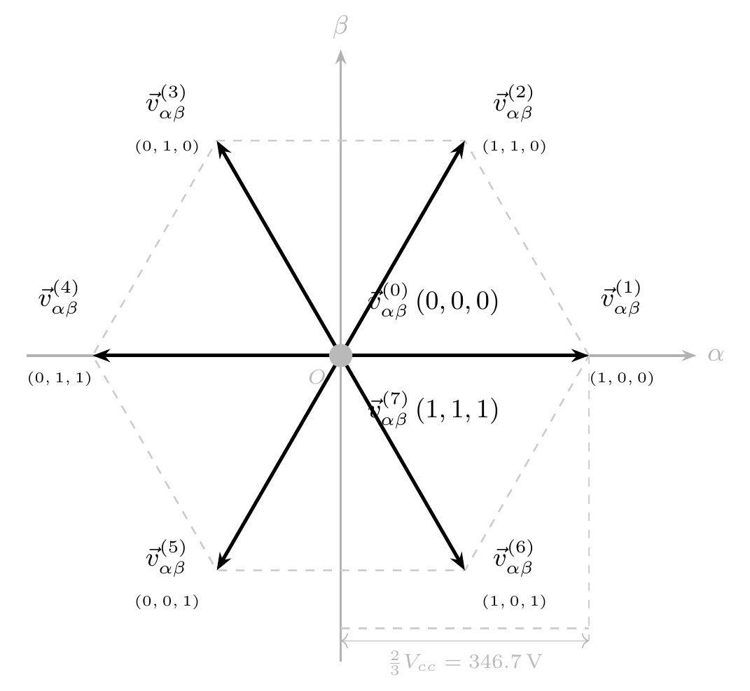
Vetores de Tensão do VSI Trifásico no Plano αβ
Hexágono de vetores de comutação de um inversor de tensão trifásico de dois níveis (V0-V7), usado em controle preditivo (FCS-MPC) e SVM.
Ver código TikZ
% figuras/tikz/vetores-vsi-plano-alphabeta.tex
% Vetores de tensão do VSI trifásico de 2 níveis no plano αβ
% IMPORTANTE: Este arquivo contém APENAS o ambiente tikzpicture.
% O ambiente figure está em 02_fundamentacao-teorica.tex.
%
% Coordenadas (escala: 1 unit = 1/3 * Vcc ≈ 173.3 V; vetores ativos = 3 units):
%   V1(100): (3, 0)     V2(110): (1.5, 2.598)   V3(010): (-1.5, 2.598)
%   V4(011): (-3, 0)    V5(001): (-1.5, -2.598)  V6(101): (1.5, -2.598)
%   V0(000), V7(111): (0, 0)     onde 2.598 ≈ 1.5*sqrt(3)

% Paleta alinhada aos gráficos Python:
%   corControle #d62728 — vetores de comutação (decisão do FCS-MPC/ARX)
\definecolor{corControle}{HTML}{d62728}
\providecommand{\vab}{\vec{v}_{\alpha\beta}}

\begin{tikzpicture}[
  vec/.style={-{Stealth[length=6pt]}, line width=1.2pt, black},
  axis/.style={-{Stealth[length=5pt]}, thick, gray!60},
  rot/.style={font=\small\bfseries, inner sep=1pt},
  lbl/.style={font=\tiny, text=black, inner sep=0.5pt},
  dim/.style={<->, thin, gray!55},
  ext/.style={dashed, gray!38, thin},
]
% ---- Eixos αβ ----
\draw[axis] (-3.8, 0) -- (4.3, 0) node[right, font=\small] {$\alpha$};
\draw[axis] (0, -3.7) -- (0, 3.7) node[above, font=\small] {$\beta$};
\node[font=\scriptsize, gray!55, below left] at (-0.05,-0.05) {$O$};

% ---- Hexágono tracejado (conecta as pontas dos 6 vetores ativos) ----
\draw[dashed, gray!40, line width=0.6pt]
  (3,0) -- (1.5,2.598) -- (-1.5,2.598) -- (-3,0)
  -- (-1.5,-2.598) -- (1.5,-2.598) -- cycle;

% ---- V1 (1,0,0): vα = 2/3·Vcc, vβ = 0 ----
\draw[vec] (0,0) -- (3,0);
\node[rot, above] at (3.40, 0.42) {$\vab^{(1)}$};
\node[lbl]        at (3.40,-0.28) {$(1,0,0)$};

% ---- V2 (1,1,0): vα = 1/3·Vcc, vβ = √3/3·Vcc — ângulo 60° ----
\draw[vec] (0,0) -- (1.5,2.598);
\node[rot] at (2.10, 3.05) {$\vab^{(2)}$};
\node[lbl] at (2.10, 2.52) {$(1,1,0)$};

% ---- V3 (0,1,0): vα = -1/3·Vcc, vβ = √3/3·Vcc — ângulo 120° ----
\draw[vec] (0,0) -- (-1.5,2.598);
\node[rot] at (-2.10, 3.05) {$\vab^{(3)}$};
\node[lbl] at (-2.10, 2.52) {$(0,1,0)$};

% ---- V4 (0,1,1): vα = -2/3·Vcc, vβ = 0 — ângulo 180° ----
\draw[vec] (0,0) -- (-3,0);
\node[rot, above] at (-3.40, 0.42) {$\vab^{(4)}$};
\node[lbl]        at (-3.40,-0.28) {$(0,1,1)$};

% ---- V5 (0,0,1): vα = -1/3·Vcc, vβ = -√3/3·Vcc — ângulo 240° ----
\draw[vec] (0,0) -- (-1.5,-2.598);
\node[rot] at (-2.10, -2.45) {$\vab^{(5)}$};
\node[lbl] at (-2.10, -2.98) {$(0,0,1)$};

% ---- V6 (1,0,1): vα = 1/3·Vcc, vβ = -√3/3·Vcc — ângulo 300° ----
\draw[vec] (0,0) -- (1.5,-2.598);
\node[rot] at (2.10, -2.45) {$\vab^{(6)}$};
\node[lbl] at (2.10, -2.98) {$(1,0,1)$};

% ---- Vetores nulos V0(000) e V7(111) — ponto preenchido na origem ----
\fill[gray!55] (0,0) circle (4pt);
\node[rot, above right, xshift=8pt, yshift=11pt] at (0,0) {$\vab^{(0)}\,(0,0,0)$};
\node[rot, below right, xshift=8pt, yshift=-11pt] at (0,0) {$\vab^{(7)}\,(1,1,1)$};

% ---- Cota de magnitude: FORA do hexágono (abaixo de y = -2.598) ----
\draw[ext] (3, 0) -- (3, -3.45);
\draw[ext, line width=0.8pt] (0, -3.30) -- (3, -3.30);
\draw[dim] (0, -3.45) -- (3, -3.45)
  node[midway, below, font=\scriptsize]
  {$\tfrac{2}{3}V_{cc} = \SI{346.7}{\volt}$};

\end{tikzpicture}